Lesson 1.10: Support Vector Machine (SVM)

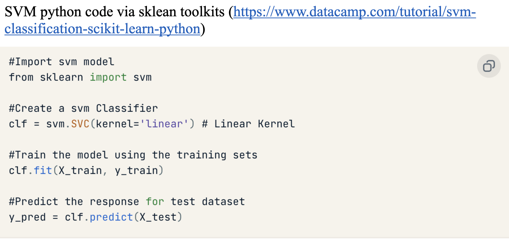
Support Vector Machines (SVM) are supervised learning models used for classification and regression. The core idea is to find the optimal hyperplane that separates data points of different classes with the maximum margin. Below is a structured breakdown of SVM concepts:

Introduction to SVM

• Discriminative Classifier: Unlike generative models (e.g., Naive Bayes), SVM directly learns the decision boundary between classes.
• Objective: Given labeled training data, SVM finds the hyperplane that maximizes the margin between the closest points of different classes (called support vectors).

Linear SVM: Separable Case

Key Concepts

• Hyperplane:
  • The decision boundary hyperplane is defined as:
    • $g(x) = \omega^T x + \omega_0 = 0$
  • For all the points above the hyperplane, $g(x) > 0$
    • $g(x) = \omega^T x + \omega_0 > 0$
  • For all the points below the hyperplane, $g(x) < 0$
    • $g(x) = \omega^T x + \omega_0 < 0$
• Margin: The distance between the hyperplane and the closest data points (support vectors).
  • Maximizing the margin improves generalization (robustness to noise).
• Support Vectors: The data points closest to the hyperplane that define the margin.

Mathematical Formulation

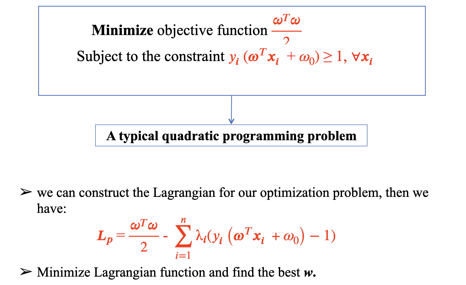
For linearly separable data, SVM solves: Objective function for hard-margin SVM: $\text{Minimize } \frac{1}{2} \|\omega\|^2$ Subject to: $y_i (\omega^T x_i + \omega_0) \geq 1 \quad \forall x_i$

• This is a quadratic programming (QP) problem.
• Solved using Lagrange multipliers (dual optimization).

Soft-Margin SVM: Non-Separable Case

In cases where data is not perfectly separable (due to noise or overlap), the hard-margin SVM (which strictly enforces fails. The soft-margin SVM addresses this by allowing some misclassifications while still maximizing the margin. When data is not perfectly separable, SVM allows some misclassifications by introducing slack variables $\epsilon_i$

Optimization Problem

• $\text{Minimize } \frac{1}{2} \|\omega\|^2 + C \sum_{i=1}^N \epsilon_i$
• Subject to:
  • $y_i (\omega^T x_i + \omega_0) \geq 1 - \epsilon_i, \quad \epsilon_i \geq 0$

Non-Linear Separable Problem in SVM

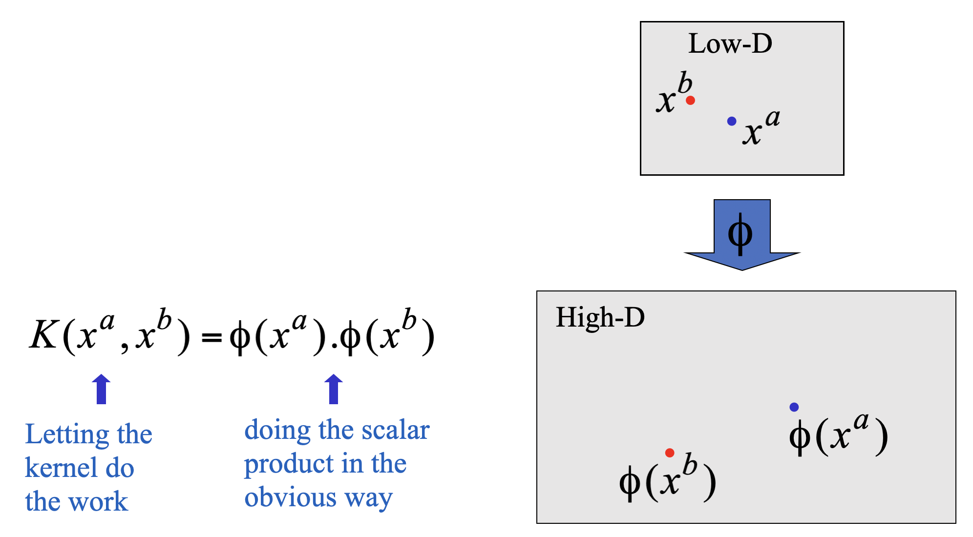
When data is not linearly separable (e.g., XOR problem, concentric circles), a linear hyperplane cannot classify it without errors. Solution: Transform the data into a higher-dimensional space where it becomes linearly separable, using the kernel trick.

1. Feature Mapping

We map the input space $\mathcal{X}$ to a higher-dimensional space $\mathcal{H}$ using a mapping function:

• $\Phi : \mathbb{R}^d \rightarrow \mathbb{R}^D \quad \text{where} \quad D \gg d$
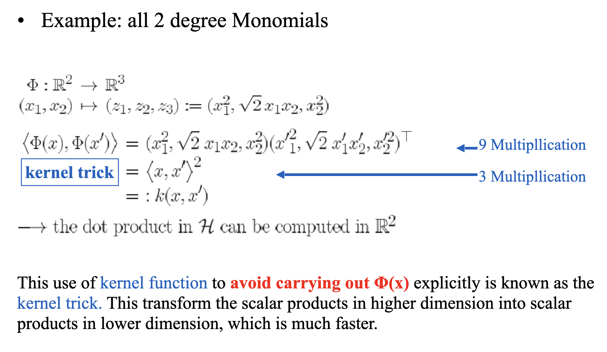
• Example (Quadratic mapping for XOR problem):
  • $\Phi(x_1, x_2) = (x_1^2, x_2^2, \sqrt{2}x_1x_2)$

2. The Kernel Trick

• If we map the input vectors into a very high-dimensional feature space, surely the task of finding the maximum-margin separator becomes computationally intractable?
• The mathematics is all linear, which is good, but the vectors have a huge number of components.
• So taking the scalar product of two vectors is very expensive.
• The way to keep things tractable is to use “the kernel trick”.
• Instead of explicitly computing $\Phi(x)$ (which can be computationally expensive), we use a kernel function:
• $K(x_i, x_j) = \langle \Phi(x_i), \Phi(x_j) \rangle$
• Efficiency Problem in Computing Feature
  • 
  • 

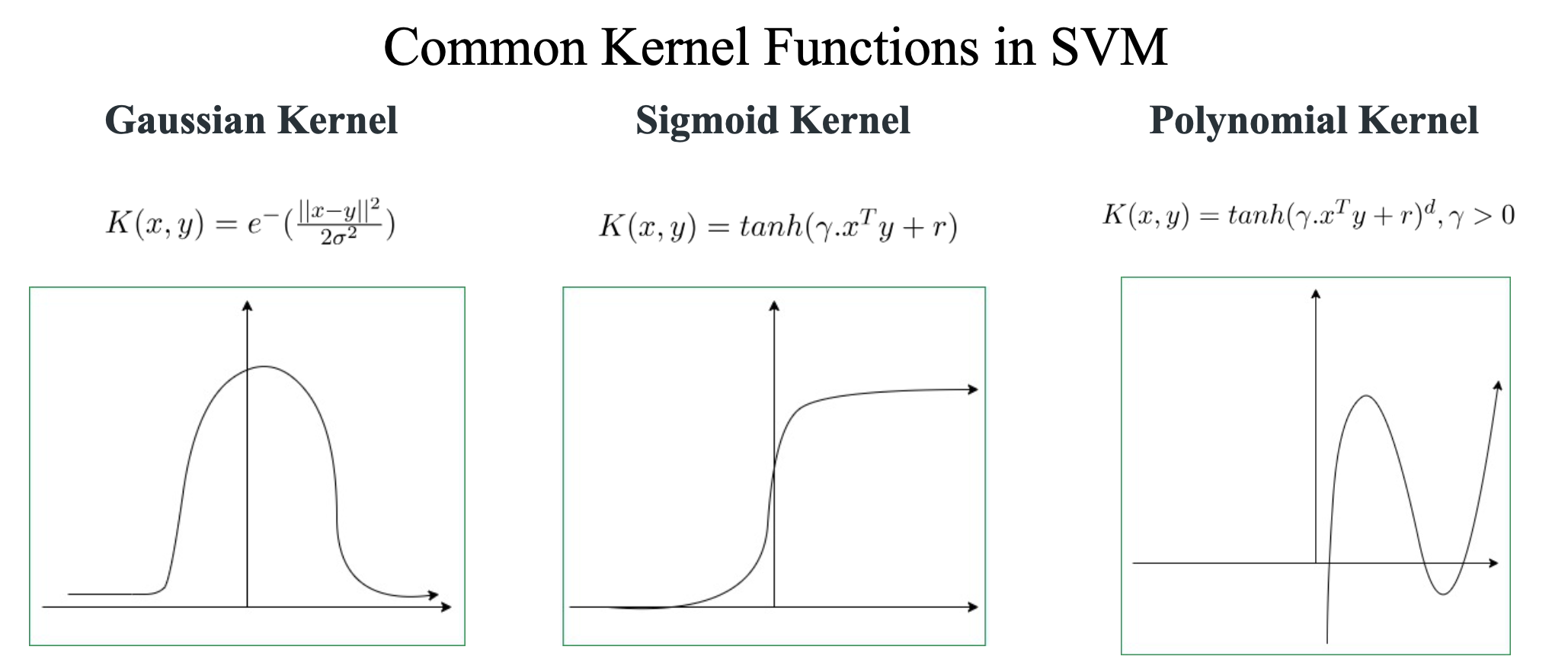
3. Common Kernel Functions

• Polynomial Kernel

  • $K(x_i, x_j) = (\gamma \langle x_i, x_j \rangle + r)^d$

• Gaussian (RBF) Kernel

  • $K(x_i, x_j) = e^{-\gamma \|x_i - x_j\|^2}$

• Sigmoid Kernel

  • $K(x_i, x_j) = \tanh(\gamma \langle x_i, x_j \rangle + r)$

Summary

1. What is a Separating Hyperplane?e

A separating hyperplane is a decision boundary that divides a dataset into distinct classes in an n-dimensional feature space. In binary classification, it acts as a surface that separates data points of one class from those of another. For a dataset to be linearly separable, there must exist at least one hyperplane that can partition the classes without any misclassification. The hyperplane is defined such that all points on one side belong to one class, while points on the other side belong to the opposite class. The goal in algorithms like SVM is to find the hyperplane that maximizes the separation (margin) between the classes, ensuring better generalization to unseen data.

2. How to Define a Separating Hyperplane?

Mathematically, a separating hyperplane in an n-dimensional space is defined by the linear equation: $\mathbf{w} \cdot \mathbf{x} + b = 0$

• w is the weight vector (normal to the hyperplane), determining its orientation.

• b is the bias term, shifting the hyperplane away from the origin.

• x represents the input feature vector.

• Key Properties:

  • Distance from a point to the hyperplane: Given a point $x_i$, its signed distance to the hyperplane is: $\frac{|\mathbf{w} \cdot \mathbf{x}_i + b|}{\|\mathbf{w}\|}$

• Classification Rule:

  • If $w⋅x+b>0$, the point is classified as Class +1.
  • If $w⋅x+b<0$, the point is classified as Class -1.

• For linearly separable data, multiple hyperplanes may exist, but SVM selects the one that maximizes the margin (distance to the nearest data points of each class).

3. What are Support Vector Machines (SVM)?

Support Vector Machines (SVM) are supervised learning models used for classification and regression. They are particularly effective for high-dimensional data and scenarios where clear margin separation is desired.

Core Concepts:

• Optimal Hyperplane: SVM finds the hyperplane that maximizes the margin between the closest points of the classes (support vectors).
• Support Vectors: These are the critical data points closest to the hyperplane, influencing its position and orientation. Removing other points does not change the hyperplane.
• Kernel Trick: For non-linearly separable data, SVM uses kernel functions (e.g., RBF, polynomial) to map data into a higher-dimensional space where separation is possible.
• Soft Margin SVM: Introduces slack variables ($ξ_i$​ ) to allow some misclassification for noisy or overlapping data.

4. How to Classify a New Example Using SVM?

Support Vector Machines classify new examples using the learned decision boundary. The process differs slightly between linear and non-linear (kernelized) SVMs:

For Linear SVM:

1. Compute the decision function:
   • $f(\mathbf{x}_{\text{new}}) = \mathbf{w} \cdot \mathbf{x}_{\text{new}} + b$
2. Apply the classification rule:
   • $\text{Class} = \begin{cases} +1 & \text{if } f(\mathbf{x}_{\text{new}}) > 0 \\ -1 & \text{if } f(\mathbf{x}_{\text{new}}) < 0 \end{cases}$
   • Where:
     • $\mathbf{w}$ is the learned weight vector
     • $b$ is the bias term
     • $\mathbf{x}_{\text{new}}$ is the new example's feature vector

For Non-Linear SVM (Kernelized):

1. Compute the decision function using support vectors:
   • $f(\mathbf{x}_{\text{new}}) = \sum_{i=1}^{N_{\text{SV}}} \alpha_i y_i K(\mathbf{x}_i, \mathbf{x}_{\text{new}}) + b$
2. Apply the same classification rule:
   • $\text{Class} = \text{sign}(f(\mathbf{x}_{\text{new}}))$
   • Where:
     • $N_{\text{SV}}$ is the number of support vectors
     • $\alpha_i$ are the learned Lagrange multipliers (non-zero only for support vectors)
     • $y_i$ are the class labels ($\pm1$) of support vectors
     • $K(\cdot,\cdot)$ is the kernel function