Lesson 2.1: Convolution Neural Network

What is a CNN?

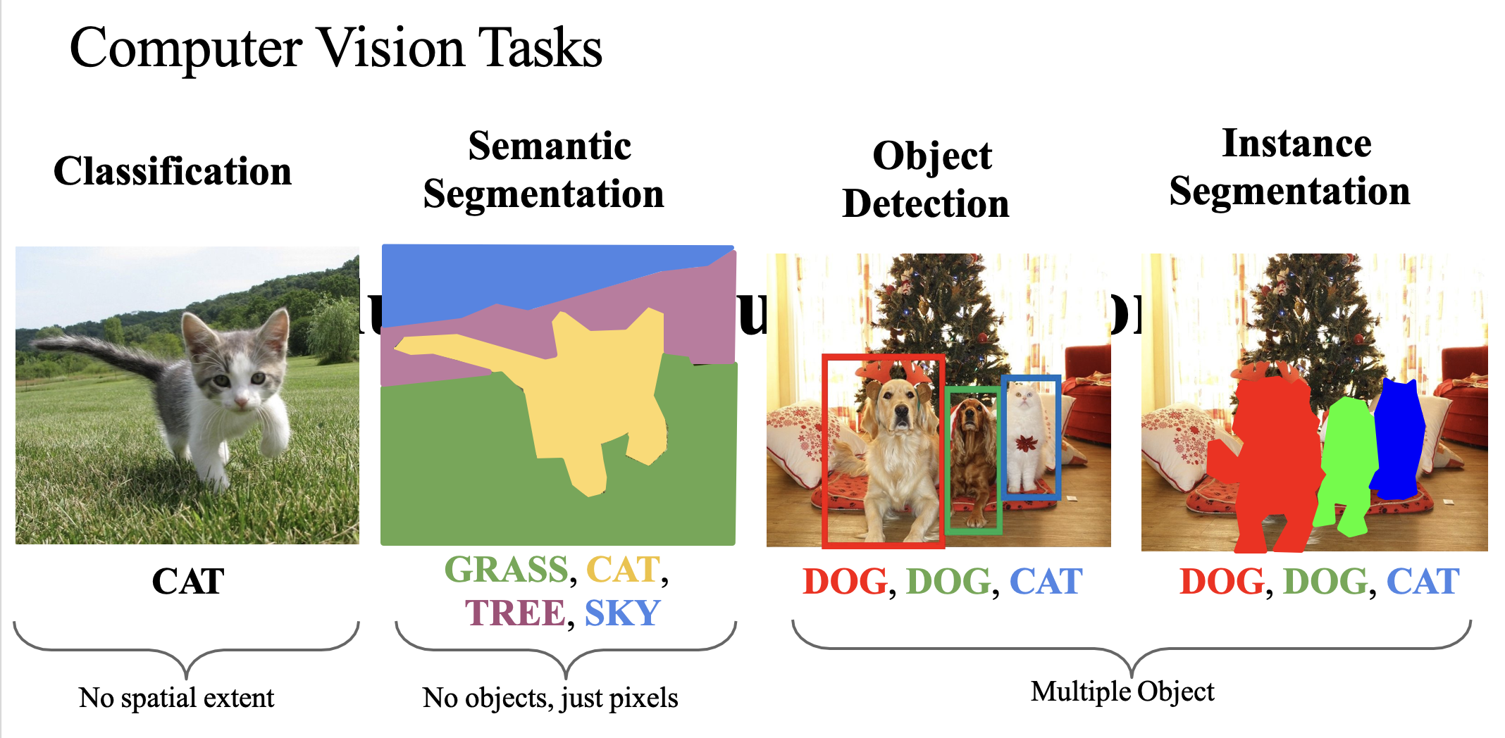
A Convolutional Neural Network (CNN) is a specialized type of artificial neural network designed for processing structured grid data like images. CNNs are particularly effective for computer vision tasks because they automatically and adaptively learn spatial hierarchies of features through backpropagation.

Why CNNs Over Traditional Neural Networks?

Traditional neural networks face several challenges when processing images:

Reduce the Number of Input Nodes
- In a traditional neural network, each pixel in an input image would be connected to each neuron in the first hidden layer. For a small 6×6 grayscale image, this means 36 input nodes. For a typical 256×256 RGB image, this would be 256×256×3 = 196,608 input nodes! This leads to:
  - Computational inefficiency - too many parameters to learn
  - Memory constraints - storing all these weights requires significant memory
  - Overfitting - with so many parameters, the model may memorize training data rather than learn general features CNNs solve this by using local connectivity - each neuron in a convolutional layer is connected only to a small region of the input (called the receptive field), dramatically reducing the number of parameters.
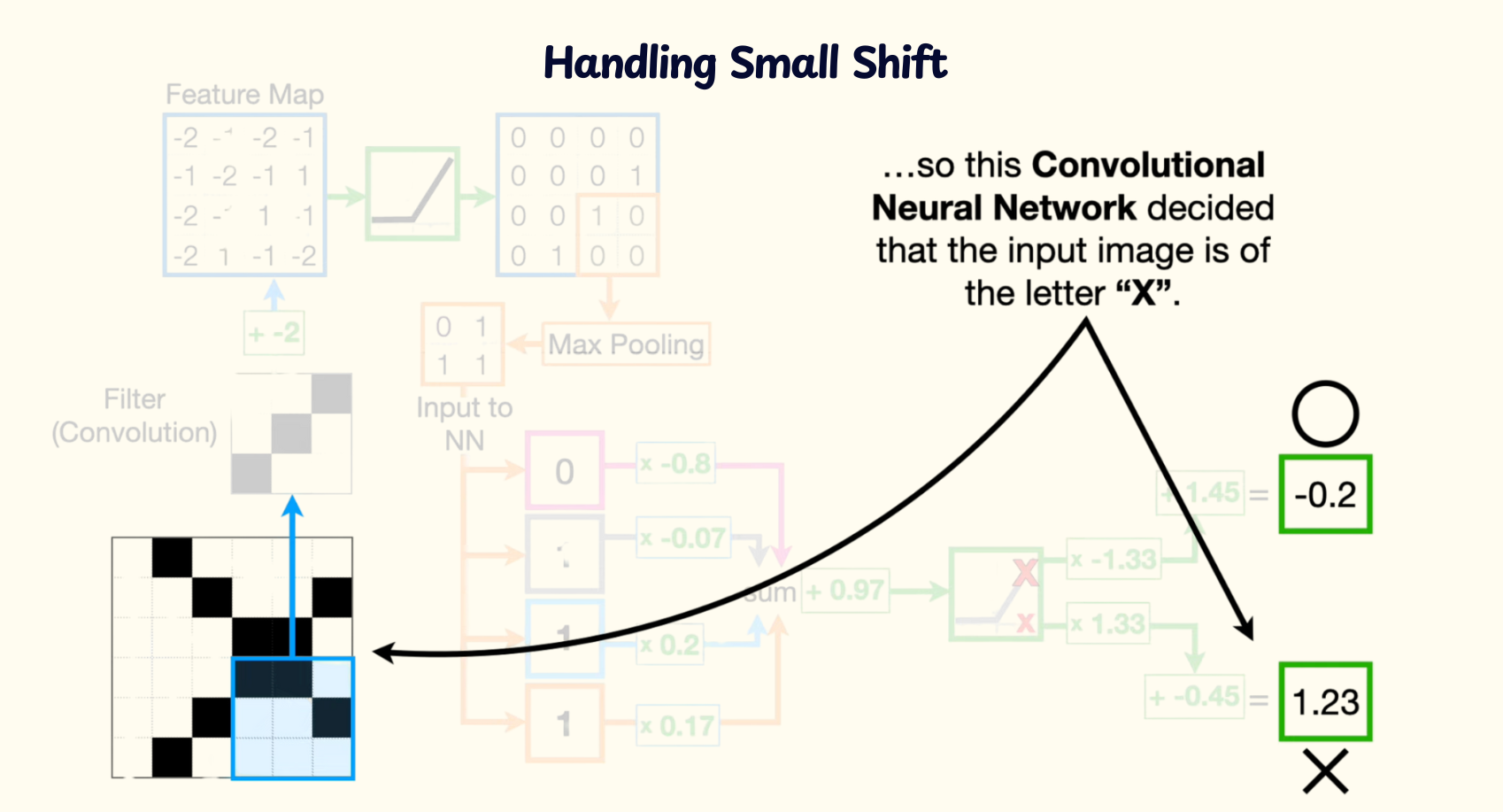
Tolerate Small Shifts in Pixel Locations
- In traditional NNs, if an object in an image shifts slightly, all the pixel values go to different input nodes, making the network see it as a completely different input. CNNs are:
  - Translation invariant - the same filter is applied across the entire image, so learned features are detected regardless of their position
  - Robust to small transformations - max pooling provides some invariance to small translations
Take Advantage of Spatial Correlation
- In images, nearby pixels are highly correlated. Traditional NNs ignore this spatial structure by flattening the image into a 1D vector. CNNs preserve and exploit this structure by:
  - Local connectivity - focusing on small regions at a time
  - Parameter sharing - using the same weights (filters) across the entire image
  - Hierarchical learning - building complex features from simple ones

Aspect	Traditional Neural Networks	Convolutional Neural Networks (CNNs)
Architecture	Fully connected layers; dense connectivity between neurons.	Convolutional + pooling layers + fully connected layers; designed for grid-like data (e.g., images).
Local Connectivity	Global connectivity: Each neuron connected to all neurons in the previous layer.	Local connectivity: Neurons in a convolutional layer connected to a small input region (receptive field).
Weight Sharing	Unique weights per neuron; no parameter sharing.	Shared weights via filters/kernels across input regions; reduces parameters.
Pooling Layers	No pooling; rely on fully connected layers for dimensionality reduction.	Include pooling (e.g., max pooling) to downsample feature maps and retain key information.
Applications	Structured data (e.g., tabular data) with simple, well-defined feature relationships	Image/video processing; tasks requiring spatial hierarchies and local pattern recognition
Parameter Efficiency	High parameter count; prone to overfitting and computational inefficiency for high-dimensional data.	Parameter-efficient due to weight sharing and local connectivity; scalable for large datasets.

Components of CNN

Filter (aka kernel)

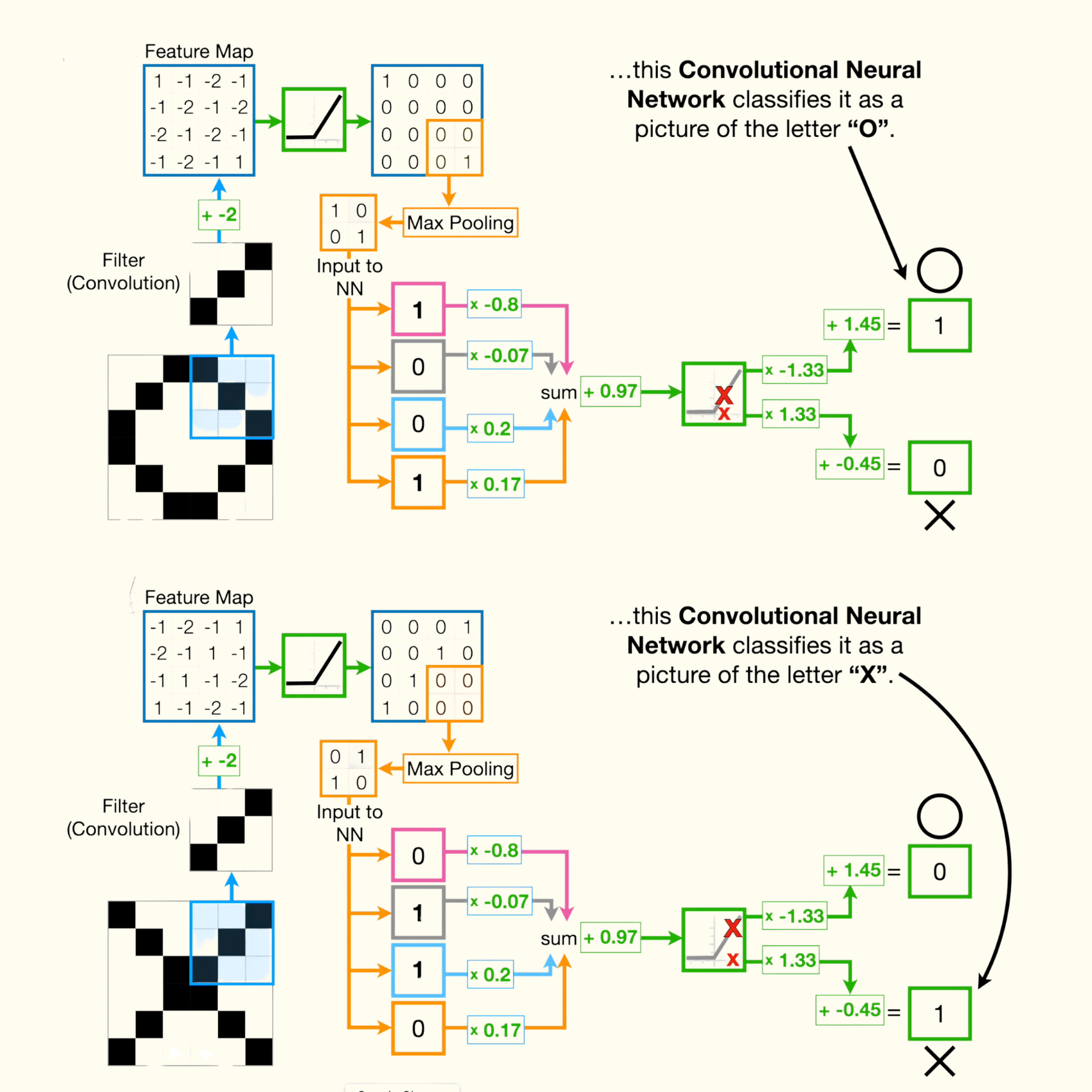
In CNN, filter is just a smaller square that is commonly 3 pixels by 3 pixels, and the intensity of each pixels is determined by backpropagation.
Before training a CNN, we start with random pixel values, and after training with backpropagation, we end up with something more useful.
We have to compute the dot product (multiply and add each pixels) between the input and the filter. We can say that the filter is convolved with the input and that is what gives Convolution Neural Network its name.
What it is: A small matrix (e.g., 3×3, 5×5) of trainable weights.
Purpose: Detects patterns (edges, textures) in input images.
How it works:
- Slides over the input image (stride=1 by default).
- Computes the dot product between filter weights and local pixel values.
Training: Starts with random values → optimized via backpropagation.

Bias Term

What it is: A single trainable value added to each filter’s output.
Purpose: Adjusts the feature map’s baseline activation.

Feature Map

What it is: Output after applying a filter to the input.
Key Idea: Highlights where the filter’s pattern (e.g., edges) appears in the image.
Example: A filter for "diagonal edges" activates on diagonal lines.

ReLU Activation

Function: ReLU(x) = max(0, x)
Purpose:
- Removes negative values (sets them to 0).
- Introduces nonlinearity, enabling complex feature learning.

Max Pooling

What it does: Downsamples the feature map to reduce size/computation.
How it works:
- Divides the feature map into windows (e.g., 2×2).
- Keeps only the maximum value in each window.
Why?: Preserves important features while reducing spatial dimensions.

Flattening

What it does: Converts the 2D feature maps into a 1D vector.
Purpose: Prepares data for the final classification layer.

Fully Connected (FC) Layer

What it is: A traditional neural network layer.
Purpose: Classifies features into labels (e.g., "cat" or "dog").
How it works:
- Takes flattened input.
- Applies weights and biases → outputs class probabilities via softmax.

Batch Normalization (BN) in CNNs

The Problem BatchNorm Solves
- In deep networks like CNNs:
  - Activations (layer outputs) can become poorly scaled (e.g., too large/small).
  - Unstable gradients make training slow or stuck.
  - Example: If inputs to a layer (y = Wx) have varying scales, weights (W) must constantly adjust, slowing convergence.
BatchNorm’s Core Idea
- Force each layer’s inputs to be zero-mean and unit-variance (per channel/dimension) for every batch during training.
- Normalize first, then scale/shift back (to preserve representational power).
How It Works (Step-by-Step)

(1) For a Batch of Activations
- Let x be a batch of activations (shape: N × C × H × W for CNNs, where C = channels).
- For each channel c in C:
(2) Compute Batch Statistics
- Mean (center the data):
  - $\mu_c = \frac{1}{N \cdot H \cdot W} \sum_{n,h,w} x_{n,c,h,w}$
- Variance (measure spread):
  - $\sigma_c^2 = \frac{1}{N \cdot H \cdot W} \sum_{n,h,w} (x_{n,c,h,w} - \mu_c)^2 + \epsilon$
- (Tiny ε avoids division by zero.)
(3) Normalize
- Center and scale each activation:
- $\hat{x}_{n,c,h,w} = \frac{x_{n,c,h,w} - \mu_c}{\sqrt{\sigma_c^2 + \epsilon}}$
- (Now x̂ has mean=0, variance=1 per channel.)
(4) Scale and Shift (Learnable Parameters)
- Introduce γ (scale) and β (shift) per channel to retain flexibility:
- $y_{n,c,h,w} = \gamma_c \hat{x}_{n,c,h,w} + \beta_c$ $y_{n, c, h, w} = γ_{c} \overset{x}{^}_{n, c, h, w} + β_{c}$
  - γ and β are learned during training.
  - If zero-mean/unit-variance hurts performance, the network can "undo" normalization by setting γ=σ, β=μ.

During Testing
- Use population estimates of μ and σ² (averaged from training batches).
- BN becomes a fixed linear transformation:

View Repository

Kernel: .venv

Building a CNN for MNIST classification in PyTorch.

In [73]:

import torch 
import torch.nn as nn 
import torch.nn.functional as F
from torch.utils.data import DataLoader
from torchvision import datasets, transforms
from torchvision.utils import make_grid

import numpy as np 
import pandas as pd
from sklearn.metrics import confusion_matrix 
import matplotlib.pyplot as plt 
%matplotlib inline

In [74]:

# Convert mnist image files into tensor of 4 Dimentions ( No. of images, height, width, color channel )
transform = transforms.ToTensor()

Training Set

Purpose: Used to train the model (adjust weights & biases via backpropagation).

Size: Usually larger (e.g., 70-80% of total data).
In MNIST: 60,000 handwritten digit images.

How it’s used:

The model learns patterns from this data.
The optimizer (e.g., SGD, Adam) updates weights to minimize loss (e.g., Cross-Entropy Loss).

train=True means this is the training set.

In [75]:

# Train Data 
train_data = datasets.MNIST(root='./cnn_data', train=True, download=True, transform=transform)

In [76]:

train_data

Out [76]:

Dataset MNIST
    Number of datapoints: 60000
    Root location: ./cnn_data
    Split: Train
    StandardTransform
Transform: ToTensor()

Test Set

Purpose: Used to evaluate the model’s performance on unseen data.

Size: Smaller (e.g., 20-30% of total data).
In MNIST: 10,000 images.

How it’s used:

After training, the model makes predictions on this set.
No weight updates happen here (with torch.no_grad() in PyTorch).
Metrics like accuracy, precision, and recall are computed.

Why Is This Important?

The test set is used to evaluate the model’s predictions against the true answers.
Without correct labels, we couldn’t measure accuracy, loss, or other metrics.

train=False means this is the test set.

In [77]:

# Test Data
test_data = datasets.MNIST(root='./cnn_data', train=False, download=True, transform=transform)

In [78]:

test_data

Out [78]:

Dataset MNIST
    Number of datapoints: 10000
    Root location: ./cnn_data
    Split: Test
    StandardTransform
Transform: ToTensor()

In [79]:

# Get the first test example
test_image, true_label = test_data[1]  
print("True Label:", true_label)  # e.g., "2"
print("Image Shape:",test_image.shape)
#plt.imshow(test_image.squeeze(), cmap='gray')  # Display the image

Out [79]:

True Label: 2
Image Shape: torch.Size([1, 28, 28])

MNIST images are 28×28 pixels and grayscale (no RGB colors).
PyTorch uses channels-first format ([channels, height, width]), unlike OpenCV (which uses [height, width, channels]).
torch.Size([1, 28, 28])

This is a 3D tensor representing a single grayscale image from the MNIST dataset.
The numbers describe:

1: Number of color channels (1 = grayscale, 3 = RGB).
28: Height of the image in pixels.
28: Width of the image in pixels.

In [80]:

# Create a small batch size for images ( suppose 10 )
train_loader = DataLoader(train_data, batch_size=10, shuffle=True)
test_loader = DataLoader(test_data, batch_size=10, shuffle=False)

train_loader = DataLoader(train_data, batch_size=10, shuffle=True)

train_data: Your MNIST training dataset (60,000 images + labels).
batch_size=10: Processes 10 images at a time (instead of all 60,000 at once).

Why? → Saves memory, speeds up training, and helps gradient updates be more stable.

shuffle=True: Randomizes the order of data in each epoch.

Why? → Prevents the model from learning the sequence of data (improves generalization).

The train_loader splits train_data into 6,000 batches (since 60,000 samples / 10 per batch = 6,000 batches).

Each batch contains:

Images tensor: Shape [10, 1, 28, 28] (batch_size, channels, height, width).
Labels tensor: Shape [10] (the correct digit for each image).

test_loader = DataLoader(test_data, batch_size=10, shuffle=False)

test_data: MNIST test dataset (10,000 images + labels).
batch_size=10: Evaluates 10 images at a time (faster than one-by-one).
shuffle=False: Keeps the original order of test data.

Why? → Ensures consistent evaluation metrics (no randomness).

The test_loader splits test_data into 1,000 batches (10,000 samples / 10 per batch).

Used for validation with torch.no_grad() (no backpropagation).

In [81]:

# Define our CNN Model 
# Describe convolutional layer and what it's doing ( 2 convolutional layers )
conv1 = nn.Conv2d(1 , 6 , 3 ,1)
conv2 = nn.Conv2d(6 , 16 , 3 , 1)

First Convolution Layer conv1 = nn.Conv2d(1, 6, 3, 1)

Input: 1 channel (grayscale pixel values).
Output: 6 channels (feature maps).
What Happens:

Six unique 3×3 filters slide over the input image.
Each filter learns to detect different low-level features (like edges at various orientations).
Example Filters Learned:

Vertical edge detector
Horizontal edge detector
Diagonal edge detectors (45° and 135°)
Blob detector
Gradient transition detector

Second Convolution Layer (conv2 = nn.Conv2d(6, 16, 3, 1))

Input: 6 channels (the edge-activated feature maps from conv1).
Output: 16 channels (higher-level features).
What Happens:

Each of the 16 filters now has a kernel shape of [6, 3, 3] (6 input channels × 3×3 spatial size).
These filters combine the 6 edge maps to detect mid-level shapes:
Corners (intersection of horizontal + vertical edges)
Curves (sequences of diagonal edges)
Junctions (T-shapes, L-shapes)

In [82]:

# Grab one MNIST record (image)
for i, (X_Train, y_train) in enumerate(train_data):
    break

X_Train.shape
x = X_Train.view(1,1,28,28)

# First Convolutional Layer (conv1)
x = F.relu(conv1(x))             # Rectified Linear Unit for activation function 
print(f'1 ----> {x.shape}')

# First Max Pooling
x = F.max_pool2d(x,2,2)         # Kernel of 2 and stride of 2 
print(f'2 ----> {x.shape}')         # 26/12=13

# Second Convolutional Layer (conv2)
x = F.relu(conv2(x))
print(f'3 ----> {x.shape}')

# Second Max Pooling
x = F.max_pool2d(x,2,2)
print(f'4 ----> {x.shape}')         # 11/2 =5.5 (round up to 5)

Out [82]:

1 ----> torch.Size([1, 6, 26, 26])
2 ----> torch.Size([1, 6, 13, 13])
3 ----> torch.Size([1, 16, 11, 11])
4 ----> torch.Size([1, 16, 5, 5])

How 5×5 Feature Maps Are Created

Your CNN transforms the input image step-by-step:

Input Image:

Shape: [1, 28, 28] (1 channel, 28×28 pixels).

After First Convolution (conv1) + Pooling:

conv1: Applies 6 filters → Output shape: [6, 26, 26].
Max-pooling (2×2, stride=2): Downsamples to [6, 13, 13].

After Second Convolution (conv2) + Pooling:

conv2: Applies 16 filters → Output shape: [16, 11, 11].
Max-pooling (2×2, stride=2): Downsamples to [16, 5, 5].

Key Calculation:

After second pooling: 11 / 2 = 5.5 → PyTorch floors to 5.
Thus, final spatial size: 5×5.

In [83]:

# Model Class
class ConvolutionalNetwork(nn.Module):
    def __init__(self):
        super().__init__()
        
        # Convolutional Layers
        self.conv1 = nn.Conv2d(1,6,3,1)     # (input_channels, output_channels, kernel_size, stride)
        self.conv2 = nn.Conv2d(6,16,3,1)    # (input_channels, output_channels, kernel_size, stride)
        
        # Fully Connected (Dense) Layers
        self.fc1 = nn.Linear(5*5*16, 120)   # In Features : 16 channels × 5 height × 5 width = 400 values per image.
        self.fc2 = nn.Linear(120, 84)
        self.fc3 = nn.Linear(84,10)
        
    def forward(self,X):
        X = F.relu(self.conv1(X))
        X = F.max_pool2d(X,2,2)         # 2*2 Kernal , Stride 2
        # Second pass
        X = F.relu(self.conv2(X))
        X = F.max_pool2d(X,2,2)         # 2*2 Kernal , Stride 2       
        # Re-view to flatten it out 
        X = X.view(-1,16*5*5)           # Negative one so that we can vary the batch size 
        # Fully Connected Layers 
        X = F.relu(self.fc1(X))
        X = F.relu(self.fc2(X))
        X = self.fc3(X)
        return F.log_softmax(X, dim=1)

Fully Connected Dense Layers

fc1: Takes flattened conv output (16 channels × 5×5 spatial dims) → 120 units

In-Features

165*5 flattens the 3D feature maps into 1D for dense layers.

16: Number of learned filters (each detects unique patterns).
5×5: Spatial compression from pooling (original 28×28 → 5×5).

Out-Features

In practice, you can treat 120 as a hyperparameter and tune it for your specific dataset, but for MNIST, it’s a reliable default.

120 is a empirically validated choice for MNIST-scale problems.
It balances model capacity and computational efficiency.
The reduction 400 → 120 → 84 → 10 ensures smooth feature compression.

fc2: 120 units → 84 units

fc3: 84 units → 10 outputs (one per MNIST digit class)

In [84]:

torch.manual_seed(41)
model = ConvolutionalNetwork()  # Creates an instance of your custom CNN class
model

Out [84]:

ConvolutionalNetwork(
  (conv1): Conv2d(1, 6, kernel_size=(3, 3), stride=(1, 1))
  (conv2): Conv2d(6, 16, kernel_size=(3, 3), stride=(1, 1))
  (fc1): Linear(in_features=400, out_features=120, bias=True)
  (fc2): Linear(in_features=120, out_features=84, bias=True)
  (fc3): Linear(in_features=84, out_features=10, bias=True)
)

torch.manual_seed(41)

Sets PyTorch's random number generator seed to 41
Ensures reproducibility by making random operations deterministic:

Weight initialization in your CNN layers
Data shuffling in DataLoader
Dropout patterns (if used)

Critical for debugging and comparing results across runs

In [85]:

criterion = nn.CrossEntropyLoss()                               # Loss Function
optimizer = torch.optim.Adam(model.parameters(), lr=0.0001)      # Optimizer

Loss Function criterion = nn.CrossEntropyLoss()

Purpose: Measures how far the model's predictions are from the true labels
What it does:

Computes the cross-entropy loss between predicted class probabilities and true labels
Automatically applies softmax to model outputs (so your model shouldn't output softmax probabilities). The purpose of Softmax function is to adjust the outputs of a convolutional neural network (CNN) so that they sum to 1
Perfect predictions → loss near 0, bad predictions → higher loss

Optimizer optimizer = torch.optim.Adam(model.parameters(), lr=0.001)

Purpose: Updates the model's weights to minimize the loss
Adam Optimizer:

Combines benefits of two other optimization methods (Momentum + RMSprop)
Automatically adjusts learning rates for each parameter
Good default choice for many deep learning tasks

Key Parameters:

model.parameters(): All trainable weights/biases in your network
lr=0.001: Learning rate (step size for weight updates) - common starting value

In [86]:

import time
start_time = time.time()

epochs = 5
train_losses = []
test_losses = []
train_acc = []
test_acc = []

for epoch in range(epochs):
    # ##########################################  TRAINING  ##########################################
    model.train()
    # Initializing Tracking Variables
    running_loss = 0.0                                      # Accumulates loss values across all batches
    correct = 0                                             # Counts how many predictions match true labels
    total = 0                                               # Counts total number of processed samples
    
    for batch_idx, (X_train, y_train) in enumerate(train_loader, 1):
        optimizer.zero_grad()                               # Clears old gradients (avoids accumulation)
        outputs = model(X_train)                            # Forward Pass: Computes predictions (outputs)
        loss = criterion(outputs, y_train)                  # Loss Calculation: Measures error between predictions and true labels
        loss.backward()                                     # Backward Pass: Computes gradients of loss w.r.t. all parameters
        optimizer.step()                                    # Optimizer Step: Updates model weights using gradients
        
        _, predicted = torch.max(outputs.data, 1)           # Gets predicted class indices (argmax)
        correct += (predicted == y_train).sum().item()      # counts correct predictions, .item() converts tensor to Python number
        total += y_train.size(0)
        running_loss += loss.item() * y_train.size(0)  # Weight by batch size
        
        if batch_idx % 600 == 0:
            print(f'Epoch: {epoch}  Batch: {batch_idx}  Loss: {loss.item():.4f}')
    
    train_loss = running_loss / len(train_loader.dataset)  # Average over SAMPLES
    train_accuracy = 100 * correct/total
    train_losses.append(train_loss)
    train_acc.append(train_accuracy)
    
    # ##########################################  TESTING  ##########################################
    
    # Setting Evaluation Mode : Disables dropout and batch normalization layers , Equivalent to model.train(False)
    model.eval()
    
    # Initializing Test Metrics
    test_loss = 0.0                                         # Accumulates loss across all test batches
    correct = 0                                             # Counts correctly classified images 
    total = 0                                               # Tracks total test images processed
    
    # Disabling Gradient Calculation : Speeds up computation by skipping gradient tracking
    with torch.no_grad():
        for X_test, y_test in test_loader:
            outputs = model(X_test)                         # Forward Pass: Computes predictions (outputs) for test batch
            loss = criterion(outputs, y_test)               # Loss Calculation: Measures prediction error
            test_loss += loss.item()                        # Loss Accumulation: Adds batch loss to running total
            # Accuracy Calculation
            _, predicted = torch.max(outputs.data, 1)       # torch.max(): Gets predicted class indices (argmax of logits)
            correct += (predicted == y_test).sum().item()   # Correct Predictions: Counts matches between predictions and true labels
            total += y_test.size(0)                         # Total Images: Tracks number of images processed (y_test.size(0) gives batch size)
    
    # Final Metrics Calculation
    test_loss = test_loss/len(test_loader)                  # Average Test Loss: Total loss divided by number of batches
    test_accuracy = 100 * correct/total                     # Test Accuracy: Percentage of correct predictions
    # Storing Results
    test_losses.append(test_loss)
    test_acc.append(test_accuracy)
    # Printing Report
    print(f'Epoch {epoch}: '
          f'Train Loss: {train_loss:.4f}, Acc: {train_accuracy:.2f}% | '
          f'Test Loss: {test_loss:.4f}, Acc: {test_accuracy:.2f}%')

total_time = (time.time() - start_time)/60
print(f'Total Training Time: {total_time:.2f} minutes')

Out [86]:

Epoch: 0  Batch: 600  Loss: 0.9863
Epoch: 0  Batch: 1200  Loss: 0.4943
Epoch: 0  Batch: 1800  Loss: 0.7394
Epoch: 0  Batch: 2400  Loss: 0.7618
Epoch: 0  Batch: 3000  Loss: 0.1825
Epoch: 0  Batch: 3600  Loss: 0.3429
Epoch: 0  Batch: 4200  Loss: 0.0989
Epoch: 0  Batch: 4800  Loss: 0.1582
Epoch: 0  Batch: 5400  Loss: 0.2032
Epoch: 0  Batch: 6000  Loss: 0.0380
Epoch 0: Train Loss: 0.5102, Acc: 84.72% | Test Loss: 0.2287, Acc: 93.37%
Epoch: 1  Batch: 600  Loss: 0.0174
Epoch: 1  Batch: 1200  Loss: 0.5581
Epoch: 1  Batch: 1800  Loss: 0.0769
Epoch: 1  Batch: 2400  Loss: 0.1098
Epoch: 1  Batch: 3000  Loss: 0.3039
Epoch: 1  Batch: 3600  Loss: 0.3141
Epoch: 1  Batch: 4200  Loss: 0.2243
Epoch: 1  Batch: 4800  Loss: 0.0077
Epoch: 1  Batch: 5400  Loss: 0.0125
Epoch: 1  Batch: 6000  Loss: 0.3291
Epoch 1: Train Loss: 0.1803, Acc: 94.60% | Test Loss: 0.1236, Acc: 96.23%
Epoch: 2  Batch: 600  Loss: 0.1914
Epoch: 2  Batch: 1200  Loss: 0.0469
Epoch: 2  Batch: 1800  Loss: 0.0150
Epoch: 2  Batch: 2400  Loss: 0.1784
Epoch: 2  Batch: 3000  Loss: 0.3768
Epoch: 2  Batch: 3600  Loss: 0.1177
Epoch: 2  Batch: 4200  Loss: 0.0451
Epoch: 2  Batch: 4800  Loss: 0.0270
Epoch: 2  Batch: 5400  Loss: 0.0320
Epoch: 2  Batch: 6000  Loss: 0.4103
Epoch 2: Train Loss: 0.1213, Acc: 96.19% | Test Loss: 0.0970, Acc: 96.88%
Epoch: 3  Batch: 600  Loss: 0.0292
Epoch: 3  Batch: 1200  Loss: 0.1116
Epoch: 3  Batch: 1800  Loss: 0.0101
Epoch: 3  Batch: 2400  Loss: 0.0050
Epoch: 3  Batch: 3000  Loss: 0.0403
Epoch: 3  Batch: 3600  Loss: 0.0714
Epoch: 3  Batch: 4200  Loss: 0.0758
Epoch: 3  Batch: 4800  Loss: 0.0034
Epoch: 3  Batch: 5400  Loss: 0.0163
Epoch: 3  Batch: 6000  Loss: 0.1479
Epoch 3: Train Loss: 0.0968, Acc: 96.95% | Test Loss: 0.0860, Acc: 97.24%
Epoch: 4  Batch: 600  Loss: 0.0533
Epoch: 4  Batch: 1200  Loss: 0.1667
Epoch: 4  Batch: 1800  Loss: 0.1596
Epoch: 4  Batch: 2400  Loss: 0.0013
Epoch: 4  Batch: 3000  Loss: 0.0797
Epoch: 4  Batch: 3600  Loss: 0.0501
Epoch: 4  Batch: 4200  Loss: 0.2365
Epoch: 4  Batch: 4800  Loss: 0.0123
Epoch: 4  Batch: 5400  Loss: 0.2015
Epoch: 4  Batch: 6000  Loss: 0.0089
Epoch 4: Train Loss: 0.0809, Acc: 97.42% | Test Loss: 0.0707, Acc: 97.59%
Total Training Time: 0.75 minutes

In [87]:

# Graph the training and test loss across epochs
plt.plot(train_losses, label='Training Loss', color='blue', marker='o')
plt.plot(test_losses, label='Test Loss', color='red', marker='x')
plt.title('Training & Test Loss Across Epochs')
plt.xlabel('Epoch')
plt.ylabel('Loss')
plt.xticks(range(len(train_losses)), range(1, len(train_losses)+1))  # Epoch numbering starts at 1
plt.legend()
plt.grid(True)
plt.show()

Out [87]:

Your training results now show healthy, realistic learning behavior for MNIST classification. Here's a detailed analysis and interpretation:

Proper Loss Dynamics:

Initial loss starts high (~0.98) and decreases gradually
No more "0.0000" loss values indicating numerical instability

Reasonable Accuracy Progression:

Train accuracy grows steadily: 84.7% → 97.4%
Test accuracy follows closely: 93.4% → 97.6%

Appropriate Generalization Gap:

Final epoch: Train 97.4% vs Test 97.6% (excellent alignment)
Shows the model isn't overfitting

In [92]:

import matplotlib.pyplot as plt

plt.figure(figsize=(12, 4))

# Loss plot
plt.subplot(1, 2, 1)
plt.plot(train_losses, label='Train Loss', marker='o')
plt.plot(test_losses, label='Test Loss', marker='x')
plt.xlabel('Epoch')
plt.ylabel('Loss')
plt.legend()

# Accuracy plot
plt.subplot(1, 2, 2)
plt.plot(train_acc, label='Train Acc', marker='o')
plt.plot(test_acc, label='Test Acc', marker='x')
plt.xlabel('Epoch')
plt.ylabel('Accuracy (%)')
plt.legend()

plt.tight_layout()
plt.show()

Out [92]:

Loss: Both curves decrease and stabilize.

Accuracy: Both curves increase and converge.

In [101]:

test_data[4221]

Out [101]:

(tensor([[[0.0000, 0.0000, 0.0000, 0.0000, 0.0000, 0.0000, 0.0000, 0.0000,
           0.0000, 0.0000, 0.0000, 0.0000, 0.0000, 0.0000, 0.0000, 0.0000,
           0.0000, 0.0000, 0.0000, 0.0000, 0.0000, 0.0000, 0.0000, 0.0000,
           0.0000, 0.0000, 0.0000, 0.0000],
          [0.0000, 0.0000, 0.0000, 0.0000, 0.0000, 0.0000, 0.0000, 0.0000,
           0.0000, 0.0000, 0.0000, 0.0000, 0.0000, 0.0000, 0.0000, 0.0000,
           0.0000, 0.0000, 0.0000, 0.0000, 0.0000, 0.0000, 0.0000, 0.0000,
           0.0000, 0.0000, 0.0000, 0.0000],
          [0.0000, 0.0000, 0.0000, 0.0000, 0.0000, 0.0000, 0.0000, 0.0000,
           0.0000, 0.0000, 0.0000, 0.0000, 0.0000, 0.0000, 0.0000, 0.0000,
           0.0000, 0.0000, 0.0000, 0.0000, 0.0000, 0.0000, 0.0000, 0.0000,
           0.0000, 0.0000, 0.0000, 0.0000],
          [0.0000, 0.0000, 0.0000, 0.0000, 0.0000, 0.0000, 0.0000, 0.0000,
           0.0000, 0.0000, 0.0000, 0.0000, 0.0000, 0.0000, 0.0000, 0.0000,
           0.0000, 0.0000, 0.0000, 0.0000, 0.0000, 0.0000, 0.0000, 0.0000,
           0.0000, 0.0000, 0.0000, 0.0000],
          [0.0000, 0.0000, 0.0000, 0.0000, 0.0000, 0.0000, 0.0000, 0.0000,
           0.0000, 0.0000, 0.0000, 0.0000, 0.0000, 0.0000, 0.0000, 0.0000,
           0.0000, 0.0000, 0.0000, 0.0000, 0.0000, 0.0000, 0.0000, 0.0000,
           0.0000, 0.0000, 0.0000, 0.0000],
          [0.0000, 0.0000, 0.0000, 0.0000, 0.0000, 0.0000, 0.0000, 0.0000,
           0.0000, 0.0000, 0.0000, 0.0000, 0.0000, 0.0000, 0.0000, 0.1451,
           0.4157, 0.5373, 0.5843, 0.0000, 0.0000, 0.0000, 0.0000, 0.0000,
           0.0000, 0.0000, 0.0000, 0.0000],
          [0.0000, 0.0000, 0.0000, 0.0000, 0.0000, 0.0000, 0.0000, 0.0000,
           0.0000, 0.0000, 0.0000, 0.0000, 0.0000, 0.0000, 0.0000, 0.5020,
           0.9922, 0.9922, 0.7098, 0.0000, 0.0000, 0.0000, 0.0000, 0.0000,
           0.0000, 0.0000, 0.0000, 0.0000],
          [0.0000, 0.0000, 0.0000, 0.0000, 0.0000, 0.0000, 0.0000, 0.0000,
           0.0000, 0.0000, 0.0000, 0.0000, 0.0000, 0.0000, 0.0314, 0.5686,
           0.9922, 0.9922, 0.6588, 0.0000, 0.0000, 0.0000, 0.0000, 0.0000,
           0.0000, 0.0000, 0.0000, 0.0000],
          [0.0000, 0.0000, 0.0000, 0.0000, 0.0000, 0.0000, 0.0000, 0.0000,
           0.0000, 0.0000, 0.0000, 0.0000, 0.0000, 0.0235, 0.5216, 0.9922,
           0.9922, 0.8627, 0.0784, 0.0000, 0.0000, 0.0000, 0.0000, 0.0000,
           0.0000, 0.0000, 0.0000, 0.0000],
          [0.0000, 0.0000, 0.0000, 0.0000, 0.0000, 0.0000, 0.0000, 0.0000,
           0.0000, 0.0000, 0.0000, 0.0000, 0.0000, 0.6667, 0.9922, 0.9922,
           0.9922, 0.9922, 0.0000, 0.0000, 0.0000, 0.0000, 0.0000, 0.0000,
           0.0000, 0.0000, 0.0000, 0.0000],
          [0.0000, 0.0000, 0.0000, 0.0000, 0.0000, 0.0000, 0.0000, 0.0000,
           0.0000, 0.0000, 0.0000, 0.1490, 0.8941, 1.0000, 0.9961, 0.9961,
           0.9961, 0.7647, 0.0000, 0.0000, 0.0000, 0.0000, 0.0000, 0.0000,
           0.0000, 0.0000, 0.0000, 0.0000],
          [0.0000, 0.0000, 0.0000, 0.0000, 0.0000, 0.0000, 0.0000, 0.0000,
           0.0000, 0.0000, 0.3647, 0.8784, 0.9922, 0.9961, 0.7922, 0.4745,
           0.9451, 0.8392, 0.0784, 0.0000, 0.0000, 0.0000, 0.0000, 0.0000,
           0.0000, 0.0000, 0.0000, 0.0000],
          [0.0000, 0.0000, 0.0000, 0.0000, 0.0000, 0.0000, 0.0000, 0.0000,
           0.0941, 0.5490, 0.9725, 0.9922, 0.8118, 0.3961, 0.0627, 0.0745,
           0.8863, 0.9922, 0.1804, 0.0000, 0.0000, 0.0000, 0.0000, 0.0000,
           0.0000, 0.0000, 0.0000, 0.0000],
          [0.0000, 0.0000, 0.0000, 0.0000, 0.0000, 0.0000, 0.0000, 0.1804,
           0.9176, 0.9922, 0.9922, 0.9922, 0.5333, 0.2000, 0.0745, 0.3333,
           0.9922, 0.9922, 0.3098, 0.0000, 0.0000, 0.0000, 0.0000, 0.0000,
           0.0000, 0.0000, 0.0000, 0.0000],
          [0.0000, 0.0000, 0.0000, 0.0000, 0.0000, 0.0000, 0.0549, 0.9098,
           0.9961, 0.9922, 0.9922, 0.9922, 0.9922, 0.9961, 0.9922, 0.9922,
           0.9922, 0.9922, 0.5804, 0.0000, 0.0000, 0.0000, 0.0000, 0.0000,
           0.0000, 0.0000, 0.0000, 0.0000],
          [0.0000, 0.0000, 0.0000, 0.0000, 0.0000, 0.0000, 0.0549, 0.9137,
           1.0000, 0.9961, 0.9961, 0.9961, 0.9961, 1.0000, 0.9961, 0.9961,
           0.9961, 0.9961, 0.3608, 0.0000, 0.0000, 0.0000, 0.0000, 0.0000,
           0.0000, 0.0000, 0.0000, 0.0000],
          [0.0000, 0.0000, 0.0000, 0.0000, 0.0000, 0.0000, 0.0000, 0.1765,
           0.5255, 0.3725, 0.3765, 0.1686, 0.4235, 0.4275, 0.2196, 0.5804,
           0.9922, 0.9922, 0.2824, 0.0000, 0.0000, 0.0000, 0.0000, 0.0000,
           0.0000, 0.0000, 0.0000, 0.0000],
          [0.0000, 0.0000, 0.0000, 0.0000, 0.0000, 0.0000, 0.0000, 0.0000,
           0.0000, 0.0000, 0.0000, 0.0000, 0.0000, 0.0000, 0.0000, 0.0745,
           0.8863, 0.9922, 0.0549, 0.0000, 0.0000, 0.0000, 0.0000, 0.0000,
           0.0000, 0.0000, 0.0000, 0.0000],
          [0.0000, 0.0000, 0.0000, 0.0000, 0.0000, 0.0000, 0.0000, 0.0000,
           0.0000, 0.0000, 0.0000, 0.0000, 0.0000, 0.0000, 0.0000, 0.0000,
           0.5020, 0.9922, 0.6078, 0.0000, 0.0000, 0.0000, 0.0000, 0.0000,
           0.0000, 0.0000, 0.0000, 0.0000],
          [0.0000, 0.0000, 0.0000, 0.0000, 0.0000, 0.0000, 0.0000, 0.0000,
           0.0000, 0.0000, 0.0000, 0.0000, 0.0000, 0.0000, 0.0000, 0.0000,
           0.4275, 0.9922, 0.3569, 0.0000, 0.0000, 0.0000, 0.0000, 0.0000,
           0.0000, 0.0000, 0.0000, 0.0000],
          [0.0000, 0.0000, 0.0000, 0.0000, 0.0000, 0.0000, 0.0000, 0.0000,
           0.0000, 0.0000, 0.0000, 0.0000, 0.0000, 0.0000, 0.0000, 0.0000,
           0.4314, 0.9961, 0.7137, 0.0000, 0.0000, 0.0000, 0.0000, 0.0000,
           0.0000, 0.0000, 0.0000, 0.0000],
          [0.0000, 0.0000, 0.0000, 0.0000, 0.0000, 0.0000, 0.0000, 0.0000,
           0.0000, 0.0000, 0.0000, 0.0000, 0.0000, 0.0000, 0.0000, 0.0000,
           0.2235, 0.9922, 0.9765, 0.0667, 0.0000, 0.0000, 0.0000, 0.0000,
           0.0000, 0.0000, 0.0000, 0.0000],
          [0.0000, 0.0000, 0.0000, 0.0000, 0.0000, 0.0000, 0.0000, 0.0000,
           0.0000, 0.0000, 0.0000, 0.0000, 0.0000, 0.0000, 0.0000, 0.0000,
           0.2510, 0.9922, 0.9961, 0.0706, 0.0000, 0.0000, 0.0000, 0.0000,
           0.0000, 0.0000, 0.0000, 0.0000],
          [0.0000, 0.0000, 0.0000, 0.0000, 0.0000, 0.0000, 0.0000, 0.0000,
           0.0000, 0.0000, 0.0000, 0.0000, 0.0000, 0.0000, 0.0000, 0.0000,
           0.1490, 0.9922, 0.9961, 0.0706, 0.0000, 0.0000, 0.0000, 0.0000,
           0.0000, 0.0000, 0.0000, 0.0000],
          [0.0000, 0.0000, 0.0000, 0.0000, 0.0000, 0.0000, 0.0000, 0.0000,
           0.0000, 0.0000, 0.0000, 0.0000, 0.0000, 0.0000, 0.0000, 0.0000,
           0.0471, 0.8902, 0.6392, 0.0471, 0.0000, 0.0000, 0.0000, 0.0000,
           0.0000, 0.0000, 0.0000, 0.0000],
          [0.0000, 0.0000, 0.0000, 0.0000, 0.0000, 0.0000, 0.0000, 0.0000,
           0.0000, 0.0000, 0.0000, 0.0000, 0.0000, 0.0000, 0.0000, 0.0000,
           0.0000, 0.0000, 0.0000, 0.0000, 0.0000, 0.0000, 0.0000, 0.0000,
           0.0000, 0.0000, 0.0000, 0.0000],
          [0.0000, 0.0000, 0.0000, 0.0000, 0.0000, 0.0000, 0.0000, 0.0000,
           0.0000, 0.0000, 0.0000, 0.0000, 0.0000, 0.0000, 0.0000, 0.0000,
           0.0000, 0.0000, 0.0000, 0.0000, 0.0000, 0.0000, 0.0000, 0.0000,
           0.0000, 0.0000, 0.0000, 0.0000],
          [0.0000, 0.0000, 0.0000, 0.0000, 0.0000, 0.0000, 0.0000, 0.0000,
           0.0000, 0.0000, 0.0000, 0.0000, 0.0000, 0.0000, 0.0000, 0.0000,
           0.0000, 0.0000, 0.0000, 0.0000, 0.0000, 0.0000, 0.0000, 0.0000,
           0.0000, 0.0000, 0.0000, 0.0000]]]),
 4)

In [102]:

# Grab just the data and reshape it, and show the image
plt.imshow(test_data[4221][0].reshape(28,28))

Out [102]:

<matplotlib.image.AxesImage at 0x16a020410>

In [105]:

# Pass the image through our model 
model.eval()
with torch.no_grad():
    new_prediction = model(test_data[4221][0].view(1,1,28,28))       # Batch size of 1 , 1 color channel , 28*28 image

In [106]:

# New prediction 
new_prediction

Out [106]:

tensor([[-2.0880e+01, -1.1725e+01, -1.0849e+01, -9.9283e+00, -7.1917e-04,
         -9.6113e+00, -2.0323e+01, -1.0270e+01, -1.4203e+01, -7.5235e+00]])

In [107]:

new_prediction.argmax()

Out [107]:

tensor(4)