Lesson 3.6: Attention

Key Issues with Recurrent Models (RNNs/LSTMs)

Linear Interaction Distance
For distant word pairs (e.g., "The cat [...] sat"), RNNs require O(sequence length) steps to interact.
Problem:
- Vanishing/exploding gradients make it hard to learn long-range dependencies.
- Linear word order is artificially enforced, while language is hierarchical (e.g., syntax trees).
Sequential Computation
- RNNs process tokens one at a time, creating a bottleneck:
  - Forward/backward passes require O(sequence length) unparallelizable steps.
  - GPUs thrive on parallel computation, but RNNs force sequential dependency.
Information Bottleneck
- The final hidden state of an encoder RNN must compress all source information into a fixed-size vector.
- Result: Loss of fine-grained details, especially for long sequences.

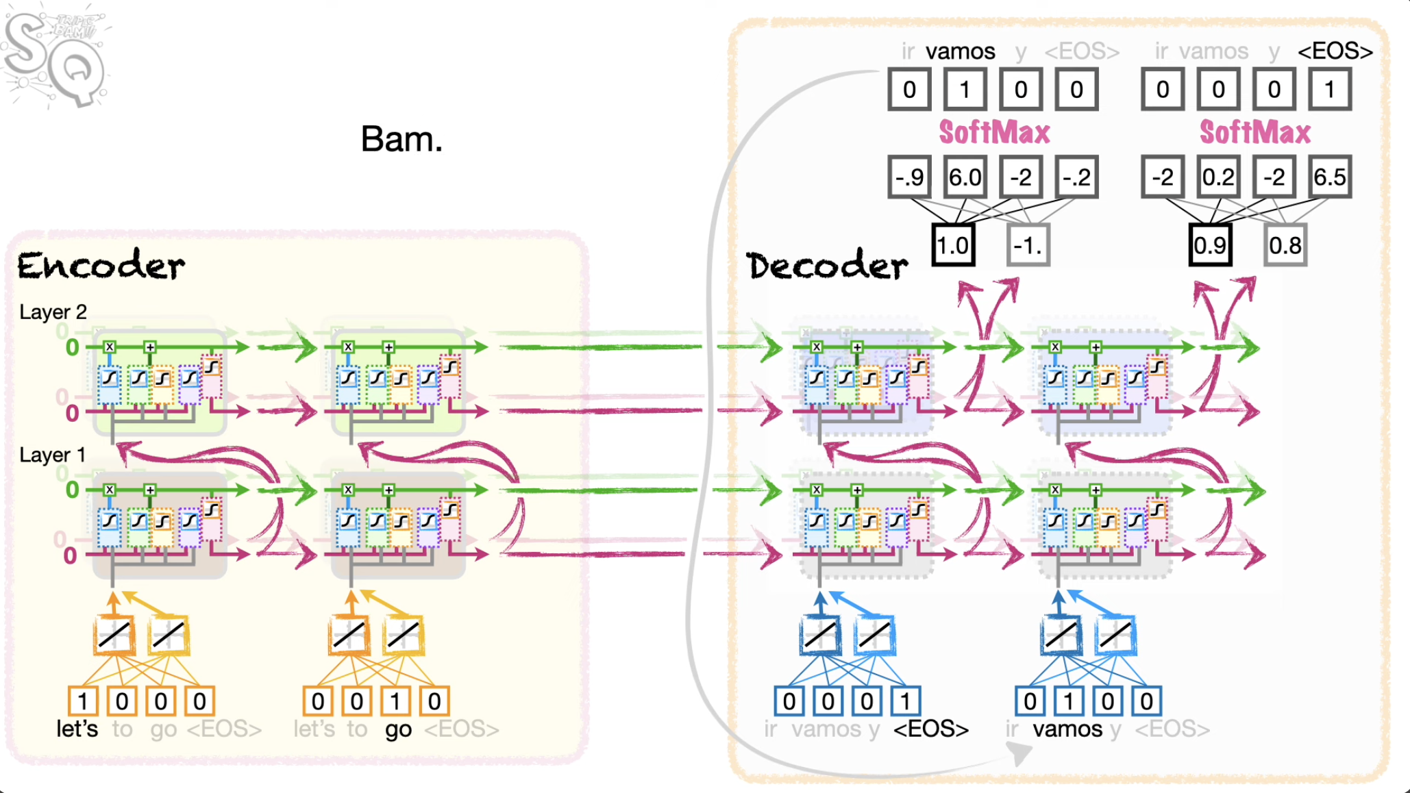
Sequence-to-Sequence (Seq2Seq) with Attention

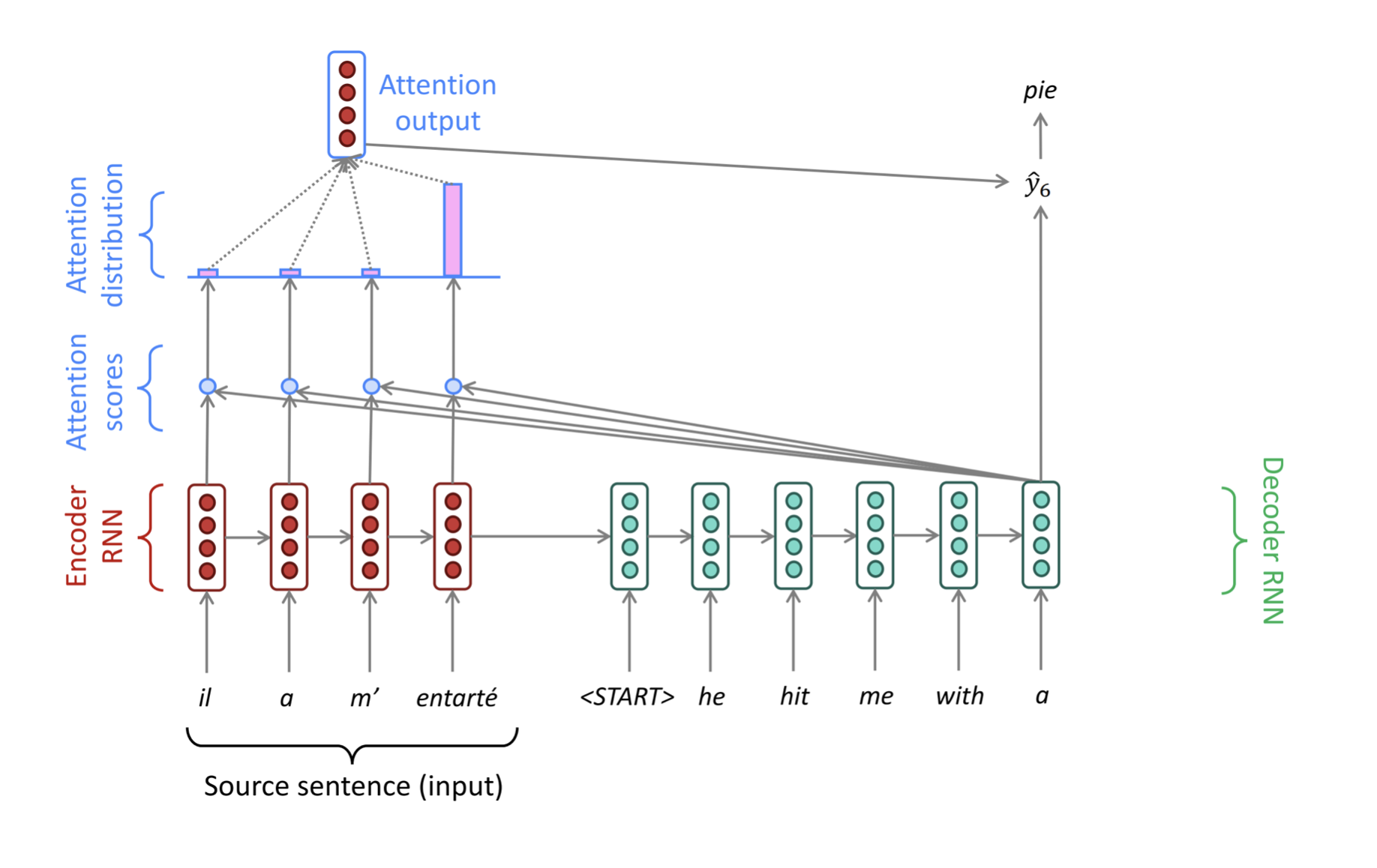
Core idea: on each step of the decoder, use direct connection to the encoder to focus on a particular part of the source sequence

Input Processing (Encoder)
- The input sequence (e.g., a sentence like "How are you?") is fed into the encoder (usually a BiLSTM or Transformer).
- Each word is converted into a vector (embedding), and the encoder processes them sequentially.
- Key steps:
  1. Embedding
    - Words → Vectors:
    - "How" → [0.2, -0.5, ...], "are" → [0.7, 0.1, ...], ...
  2. Hidden States:
    - The encoder generates a hidden state $h_i$ for each word, capturing its context:
    - h₁ ("How"), h₂ ("are"), h₃ ("you"), h₄ ("?")
    - Output: A sequence of encoder states $h_1,h_2,h_3,h_4$
Decoder Initialization
- The decoder (usually an LSTM) starts with:
- Initial hidden state: Set to the encoder’s last state $s_0 = h_4$
- First input: A special <SOS> (Start-of-Sequence) token or also <EOS>.
- Purpose: Prepares the decoder to generate the first word of the output (e.g., a translation).
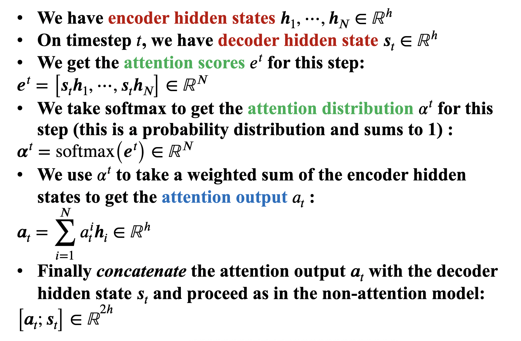
Decoder Step with Attention (Iterative Process)
- For each output word (e.g., generating Spanish "¿Cómo estás?"):
- Step 3.1: Compute Attention Weights
  - The decoder calculates how much to "focus" on each encoder state $h_i$ for the current step.
  - Uses the decoder’s previous hidden state $(s_t - 1)$ and all the encoder states $h_i$ .
  - Scores: For each encoder state $h_i$ $h_{i}$ :
    - $e_{ti} = \text{score}(s_{t-1}, h_i) = v^T \tanh(W[s_{t-1}; h_i] + b)$
  - Weights: Softmax turns scores into probabilities
    - $\alpha_{ti} = \frac{\exp(e_{ti})}{\sum_j \exp(e_{tj})}$
    - Example: For the decoder step generating "Cómo", $α_t1$ (for "How") might be 0.9.
- Step 3.2: Create Context Vector
  - The encoder states are weighted by $α_ti$ and summed:
  - $c_t = \sum_i \alpha_{ti} h_i$
  - Example: If generating "Cómo", $c_t ≈ h_1$ (since "How" → "Cómo").
- Step 3.3: Update Decoder State
  - Previous hidden state $(s_t - 1)$
  - Context vector $c_t$
  - Previously predicted word (or <SOS> for the first step).
  - $s_t = \text{LSTM}([y_{t-1}; c_t], s_{t-1})$
- Step 3.4: Predict Next Word
  - The decoder predicts a probability distribution over the output vocabulary:
  - $p(y_t) = \text{softmax}(W_o s_t + b_o)$
- Repeat: Steps 3.1 - 3.4 until <EOS> (End-of-Sequence) is generated.

Attention is Great

Attention significantly improves NMT performance
- It’s very useful to allow decoder to focus on certain parts of the source
Attention provides a more “human-like” model of the MT process
- You can look back at the source sentence while translating, rather than needing to remember it all
Attention solves the bottleneck problem
- Attention allows decoder to look directly at source; bypass bottleneck
Attention helps with the vanishing gradient problem
- Provides shortcut to faraway states
Attention provides some interpretability
- By inspecting attention distribution, we see what the decoder was focusing on
- We get (soft) alignment for free!
- This is cool because we never explicitly trained an alignment system
- The network just learned alignment by itself

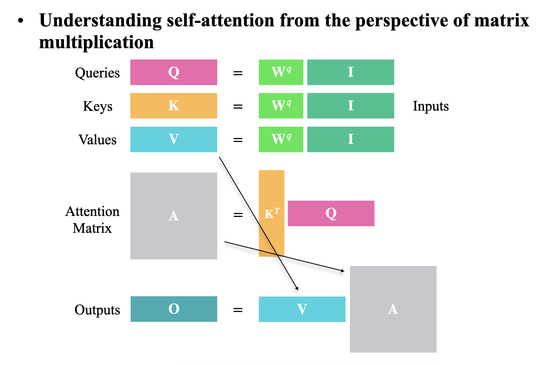
Attention in equations

Why Attention Solves Parallelization & Bottleneck Problems

Parallel Computation of Attention Scores
- All attention scores can be computed simultaneously for the entire sequence:
- $\text{Scores: } e_{ij} = \frac{q_i^T k_j}{\sqrt{d_k}} \quad \forall i,j$
- (Where $q_i$ = query for position $i$ , $k_j$ = key for position $j$ )
Eliminating Sequential Bottlenecks
- Unlike RNNs which require O(N) sequential operations, attention computes all positions at once:
- $\text{Attention}(Q,K,V) = \text{softmax}\left(\frac{QK^T}{\sqrt{d_k}}\right)V$ $Attention (Q, K, V) = softmax (\frac{Q K ^{T}}{d _{k}}) V$
  - $Q,K,V$ are matrices containing all queries/keys/values
  - Single matrix multiplication replaces sequential processing
Constant Interaction Distance
- Any two words can interact directly in one layer:
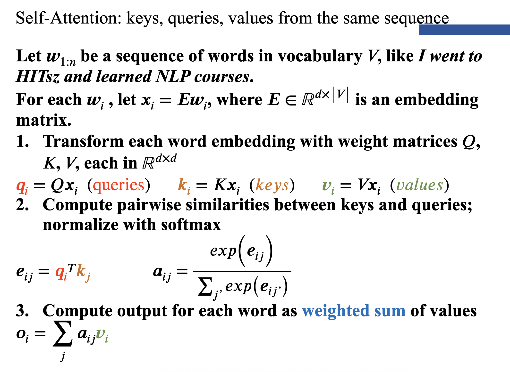
- $\text{Interaction distance} = O(1) \text{ (not } O(N) \text{ like RNNs)}$
Self-Attention Within a Sentence
- The same mechanism works for encoder self-attention:
- $h_i' = \sum_{j=1}^N \alpha_{ij} W_v h_j \quad \text{where } \alpha_{ij} = \text{softmax}(e_{ij})$ $h_{i}^{'} = \sum_{j = 1}^{N} α_{ij} W_{v} h_{j} where α_{ij} = softmax (e_{ij})$
  - Each position $i$ attends to all positions $j$ in parallel
  - No information bottleneck - all positions remain accessible

Why This Matters

Training Speed: Attention layers utilize GPU parallelism fully
Model Quality: Direct access to all positions helps learn complex dependencies
Scalability: Constant path length regardless of sequence length

Basic Attention Framework

For query q, values V = ${v_1, ..., v_N}$ , and keys K = ${k_1, ..., k_N}$ :

Attention Scores: $e_i = \text{score}(q, k_i)$
Attention Distribution (softmax): $\alpha_i = \frac{\exp(e_i)}{\sum_{j=1}^N \exp(e_j)}$
Context Vector (weighted sum): $c = \sum_{i=1}^N \alpha_i v_i$

Common Attention Variants

Dot-Product Attention
- $e_i = q^T k_i$
- Pros: Computationally efficient.
- Cons: Scores can grow large in magnitude ( $\Rightarrow$ unstable gradients).
Scaled Dot-Product (Transformer Attention)
- $e_i = \frac{q^T k_i}{\sqrt{d_k}}$
- Why scale?: Prevents gradient saturation when $d_k$ (key dimension) is large.
Additive Attention
- $e_i = v^T \tanh(W_q q + W_k k_i + b)$
- Pros: More expressive.
- Cons: Slower (extra parameters $W_q, W_k, v$ ).
Multi-Head Attention
- $\footnotesize{ \text{head}_i = \text{Attention}(W_q^i q, W_k^i K, W_v^i V) , \text{MultiHead}(q,K,V) = W_o [\text{head}_1; ...; \text{head}_h] }$
- Key idea: Parallel attention heads capture different relationships.
Self-Attention (Special Case)
- When queries, keys, and values come from the same sequence ( $q_i, k_i, v_i$ are all linear transforms of input $x_i$ ):

More general definition of attention:

Given a set of vector values, and a vector query, attention is a technique to compute a weighted sum of the values, dependent on the query.
Intuition:
- The weighted sum is a selective summary of the information contained in the values, where the query determines which values to focus on.
- Attention is a way to obtain a fixed-size representation of an arbitrary set of representations (the values), dependent on some other representation (the query).
Upshot:
- Attention has become the powerful, flexible, general way pointer and memory manipulation in all deep learning models.

Barriers and Solutions for Self-Attention as a Building Block

Barrier 1: Lack of Inherent Order

Problem:
- Self-attention treats inputs as a bag of words—it has no built-in notion of position.
- For example: "Dog bites man" vs. "Man bites dog" would have identical representations without positional cues.
Solution: Positional Encodings Inject position information into the input embeddings. Two main approaches:

Sinusoidal Positional Encodings

Idea: Use fixed, periodic sinusoidal functions to encode positions.
Equation:
- For position $pos$ and dimension $i$
- $PE_{(pos, 2i)} = \sin\left(\frac{pos}{10000^{2i/d_{\text{model}}}}\right) \\ PE_{(pos, 2i+1)} = \cos\left(\frac{pos}{10000^{2i/d_{\text{model}}}}\right)$
- (Where $d_{model}$ = embedding dimension)
- Intuition:
  - Periodicity: Different frequencies capture varying scales of positional relationships.
  - Extrapolation: Theoretically generalizes to longer sequences (though rarely works in practice).
- Pros:
  - No learned parameters (fixed).
  - Periodicity may help generalization.
- Cons:
  - Not adaptive to data.
  - Fails to extrapolate reliably.

Learned Positional Embeddings
- Idea: Treat positions as learnable vectors (like word embeddings).
- Equation:
  - $PE = \begin{bmatrix} p_1 & p_2 & \dots & p_N \end{bmatrix}^T \quad \text{(Learnable matrix)}$
  - Each $p_i ∈R d_{model}$ is trained via backpropagation.
- Pros:
  - Adapts to data (e.g., learns syntax-aware positions).
  - Simpler implementation.
- Cons:
  - Cannot extrapolate beyond trained sequence length $N$ .
  - Requires more memory.
- Used By: Most modern Transformers (e.g., BERT, GPT).

How Positional Encodings Are Integrated

Step: Add (or concatenate) positional embeddings to input word embeddings:
- $x_i' = x_i + p_i \quad \text{(Most common)} \\ \text{or} \quad x_i' = [x_i; p_i]$
Why Addition?
- Empirically works better than concatenation (fewer parameters, similar performance).
- The Transformer’s self-attention can "disentangle" position and content implicitly.

Barrier 2: Lack of Nonlinearity in Self-Attention

Problem: Self-attention is fundamentally a weighted average of value vectors. Without nonlinearities, stacking multiple self-attention layers is equivalent to a single averaged representation:
$\text{SelfAttention}(X) = \text{softmax}\left(\frac{XW_Q (XW_K)^T}{\sqrt{d_k}}\right) XW_V$
No "deep learning magic": Pure linear transformations + softmax (which is monotonic) cannot learn complex hierarchical features.
Why: Stacking $N$ $N$ linear self-attention layers reduces to a single linear operation:
- $\text{SelfAttention}^N(X) = X \cdot (W_Q W_K^T W_V)^N$
- (No new representational power is gained!)
Solution: Add Feedforward Networks (FFNs)
- Fix: Apply a position-wise FFN after each self-attention layer to introduce nonlinearity.
- Equation: For each output vector $h_i$ $h_{i}$ from self-attention:
  - $h_i' = \text{ReLU}(h_i W_1 + b_1) W_2 + b_2$
  - (Where $W_1 ∈ \mathbb{R}^{d*d_{ff}} \text{and} W_2 ∈ \mathbb{R}^{d_{ff}*d}$ )
- Key Properties:
  - Nonlinearity: ReLU breaks linearity, enabling hierarchical feature learning.
  - Position-Wise: Applied independently to each token (parallelizable).
- Why This Works
  - Self-Attention: Mixes information across positions (weighted average).
  - FFN: Processes each position independently with nonlinear transformations.
    - Think of it as a "per-token MLP" that refines features.
  - Analogy:
    - Self-attention = "global communication" (tokens talk to each other).
    - FFN = "local computation" (each token thinks independently).

Barrier 3: Preventing Future Peeking in Decoders

Problem: In tasks like language modeling or machine translation, the model must predict the next word without seeing future tokens.
Example: When predicting "estás" in "¿Cómo ___?", the model shouldn’t see "estás" or "?" in the input.
Challenge: Standard self-attention attends to all tokens in parallel → leaks future info.
Solution: Masked Self-Attention
- Artificially set attention weights to 0 for future positions.
Step-by-Step Implementation
1. Compute Attention Scores (as usual):
  - $e_{ij} = \frac{q_i^T k_j}{\sqrt{d_k}}$
2. Apply Mask (for decoder at position i):
  - Effect: Future tokens get exp(-∞) = 0 after softmax
  - $\tilde{e}_{ij} = \begin{cases} e_{ij} & \text{if } j \leq i \quad \text{(past/present)} \\ -\infty & \text{if } j > i \quad \text{(future)} \end{cases}$
3. Compute Attention Output:
  - $\alpha_{ij} = \text{softmax}(\tilde{e}_{ij}) \\ c_i = \sum_{j=1}^i \alpha_{ij} v_j$
Why This Works
- Parallelization: All positions computed simultaneously (unlike RNNs), but future tokens are masked.
- Causality: Each token only attends to itself and prior tokens.
- Efficiency: Implemented via a lower-triangular mask (see code below).

The 4 Essential Components of a Self-Attention Building Block

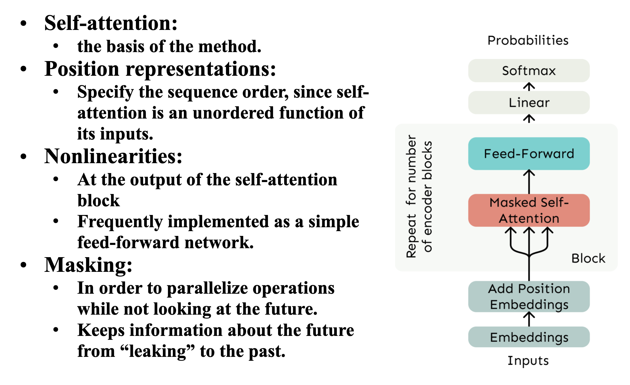
Self-Attention (Core Mechanism)
- Allows each token to dynamically focus on relevant parts of the sequence.
- Computes relationships between all pairs of tokens.
- $\text{Attention}(Q,K,V) = \text{softmax}\left(\frac{QK^T}{\sqrt{d_k}}\right)V$ $Attention (Q, K, V) = softmax (\frac{Q K ^{T}}{d _{k}}) V$
  - Queries (Q): What each token is looking for.
  - Keys (K): What each token contains.
  - Values (V): Actual content being retrieved.
- Without self-attention, the model has no way to learn contextual relationships between tokens.
Position Representations
- Injects information about token order since self-attention is permutation-equivariant.
- Sinusoidal Encoding (Fixed):
- Learned Embeddings (Trainable):
- Implementation: x = token_embeddings + position_embeddings # Additive (most common)
Nonlinearities (Feed-Forward Network)
- Introduces nonlinear transformations to enable hierarchical feature learning.
- $\text{FFN}(x) = \text{ReLU}(xW_1 + b_1)W_2 + b_2$
- Why It's Needed: Pure self-attention is just weighted averaging - FFNs add representational power.
Masking (for Autoregressive Tasks)
- Prevents the model from "cheating" by looking at future tokens during training.
- Why It's Needed: Ensures predictions at position i depend only on tokens 1 to i-1 (crucial for language modeling).

How These Components Work Together

Input: Token embeddings + positional encodings.
Self-Attention: Computes contextual relationships.
Masking: Optional - applied in decoder for autoregressive tasks.
FFN: Further processes each token's representation.