Lesson 1.12: Unsupervised Learning

Unsupervised learning is a type of machine learning that deals with identifying patterns within the data without the guidance of a known outcome or label. This approach is invaluable for discovering the underlying structure of the data, highlighting similarities, and distinguishing differences when the classification criteria are not previously known. Two fundamental techniques in unsupervised learning are Dimension Reduction and Clustering.

Part 1: Dimensionality Reduction in Unsupervised Learning

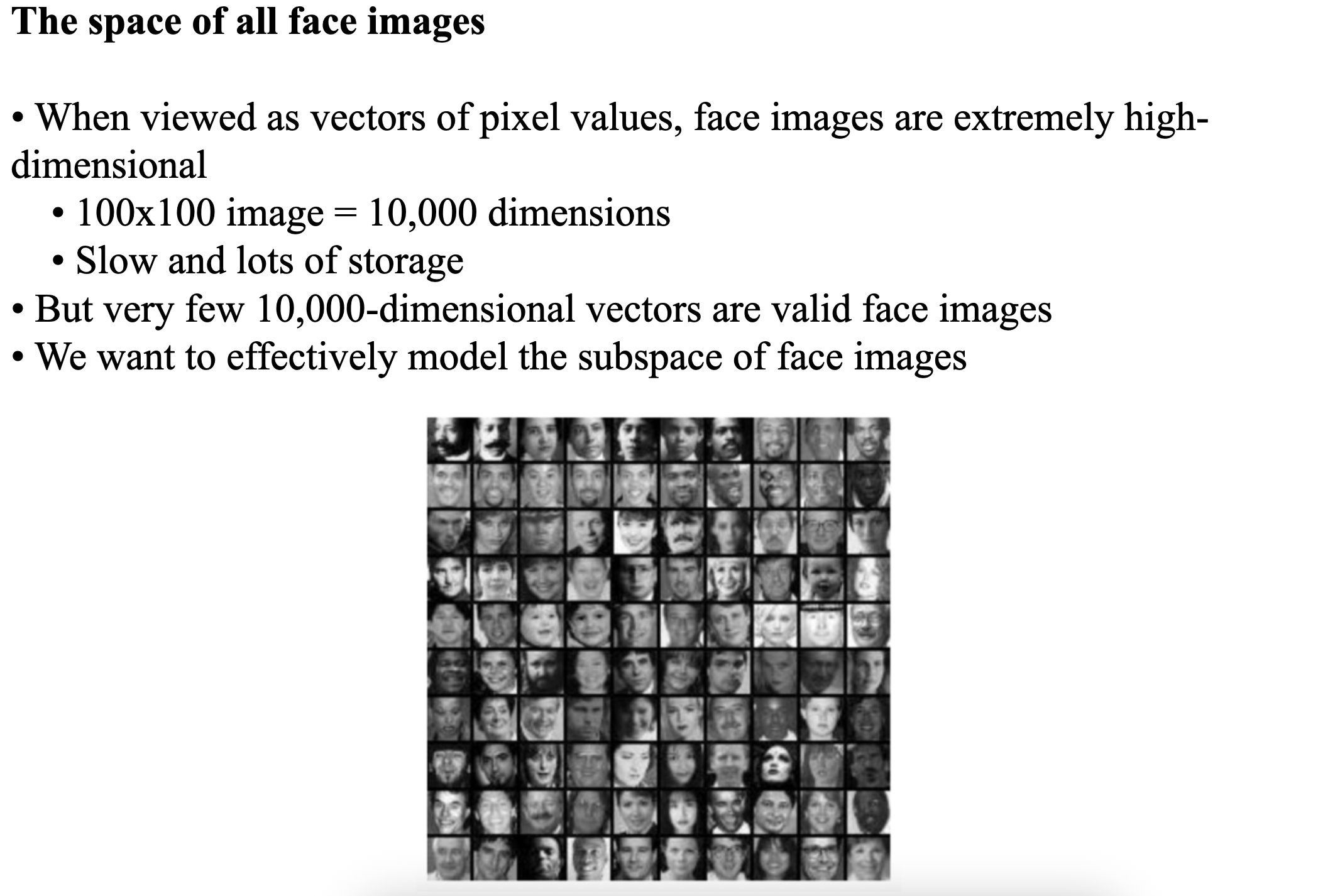
Dimensionality reduction aims to transform high-dimensional data into a lower-dimensional space while preserving as much meaningful information as possible. Here’s a structured breakdown of the key concepts:

Empirical Mean Vector

Represents the average of data points across each dimension.
Formula:
- $\mathbf{\mu} = \frac{1}{N} \sum_{i=1}^N \mathbf{x}_i$
- where $x_i$ is a data point and $N$ is the number of samples.

Empirical Variance

Measures the average squared deviation from the mean.
Formula:
- $\text{Var}(X) = \frac{1}{N} \sum_{i=1}^N (x_i - \mu)^2$

Covariance

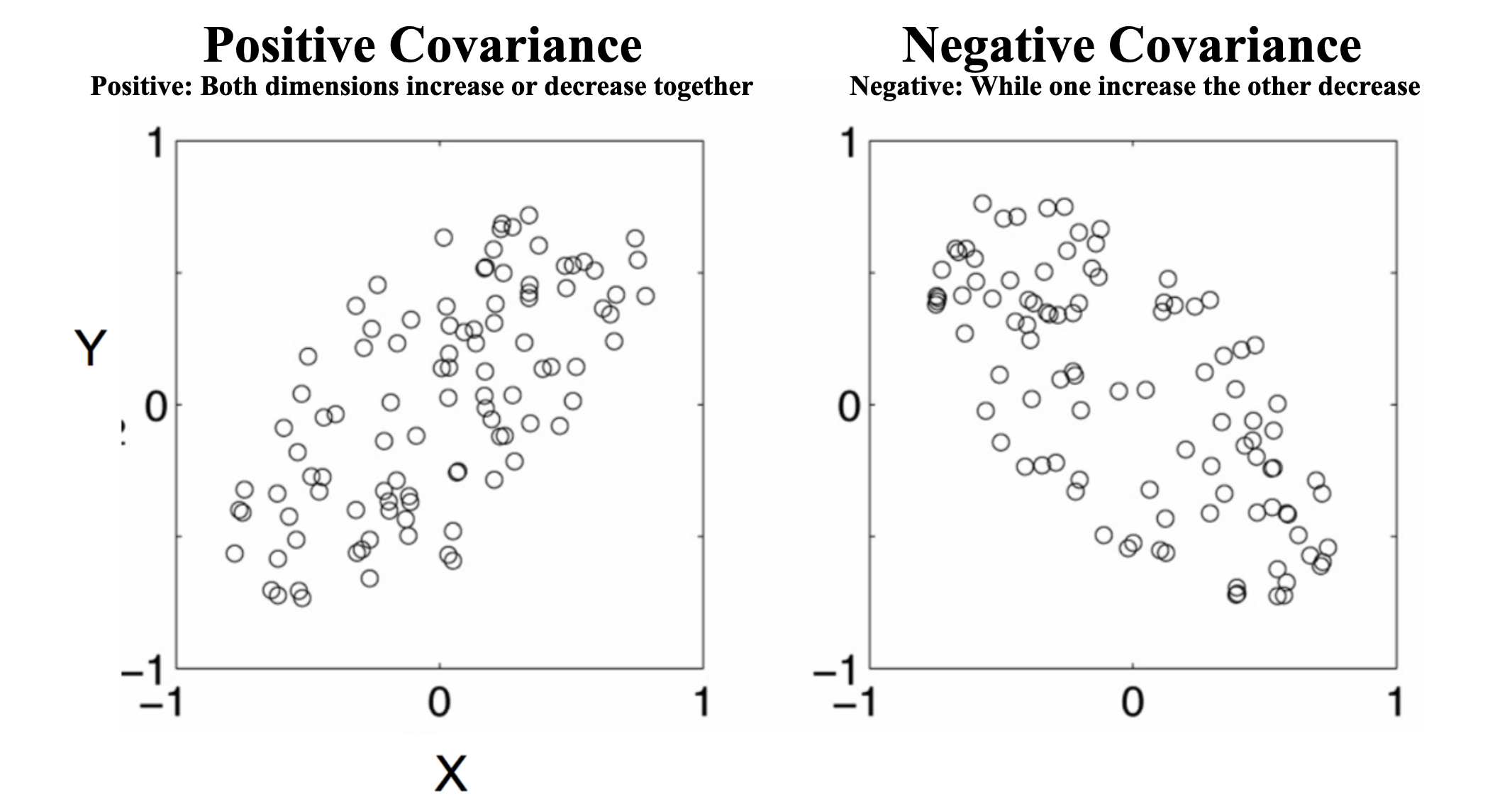
Quantifies the relationship between two dimensions:
- Positive Covariance: Both dimensions increase/decrease together.
- Negative Covariance: One increases while the other decreases.
- Zero Covariance: No linear relationship.
$\text{Cov}(X, Y) = \frac{1}{N} \sum_{i=1}^N (x_i - \mu_X)(y_i - \mu_Y)$
Variance is a special case: $\text{Cov}(X, Y) = \text{Var}(X)$

Goal of Dimensionality Reduction

Compress data from D-dimensions to K-dimensions $(K<D)$ .
Minimize reconstruction error: The difference between original data and its compressed representation.

Linear Projection (2D → 1D)

A linear projection transforms data from a higher-dimensional space (e.g., 2D) to a lower-dimensional space (e.g., 1D) using a linear transformation (matrix multiplication).

Input: A dataset in 2D space (points: $(x_1,x_2,x_3,...,x_n)$ ).
Output: A 1D representation (scalar values $(z_1,z_2,z_3,...z_n)$ )
Objective: Reduce data from 2D to 1D while minimizing information loss (reconstruction error).
Step 1: Mean-Centering the Data
- First, subtract the empirical mean from all data points to center the data around the origin:
- $\mathbf{x}' = \mathbf{x} - \mathbf{\mu}, \quad \mathbf{\mu} = \left( \frac{1}{n} \sum_{i=1}^n x_i, \frac{1}{n} \sum_{i=1}^n y_i \right)$
- Why? Ensures the projection is invariant to translation.
Step 2: Choose a Projection Direction $(w)$
- Purpose: Select a direction $w$ along which to project the data.
- Options:
  - **Manual Choice **(e.g., x-axis: $w =(1,0)$ )
  - PCA-Based Choice (optimal direction maximizing variance)
    - Compute covariance matrix.
      - $\mathbf{C} = \frac{1}{n} \mathbf{X}'^T \mathbf{X}'$
    - Find eigenvectors of $C$ $C$ . The eigenvector with the largest eigenvalue gives the best projection direction.
      - $\mathbf{w} = \text{argmax}_{\|\mathbf{w}\|=1} \mathbf{w}^T \mathbf{C} \mathbf{w}$
Step 3: Project Data onto $w$
- Purpose: Transform 2D data into 1D by computing projections.
- Formula : $z_i = \mathbf{w}^T \mathbf{x}'_i = w_1 x'_i + w_2 y'_i$
Step 4: Reconstruct Data in 2D
- Purpose: Map the 1D projections back to 2D to assess information loss.
- $\mathbf{\hat{x}}'_i = z_i \mathbf{w}$
- $\mathbf{\hat{x}}_i = \mathbf{\hat{x}}'_i + \mathbf{\mu}$ $\hat{x}_{i} = \hat{x}_{i}^{'} + μ$
  - $\mathbf{\hat{x}}'_i$ Reconstructed centered point , $\mathbf{\hat{x}}_i$ Reconstructed original point
Step 5: Calculate Reconstruction Error (MSE)
- Purpose: Measure how much information is lost in projection.
- $\text{MSE} = \frac{1}{n} \sum_{i=1}^n \|\mathbf{x}_i - \mathbf{\hat{x}}_i\|^2$
- (In general, MSE > 0 if projection is not perfect.)
Step 6: Optimize $w$ to Minimize Error
- Purpose: Find the best $w$ that minimizes reconstruction error.
- Method:
  - PCA Solution: $\mathbf{w} = \text{Eigenvector}(\mathbf{C}) \quad \text{(largest eigenvalue)}$
  - Gradient Descent (Alternative Approach)

Principal Component Analysis

Goal: Find K-dim projection that best preserves variance.
Compute eigenvectors and eigenvalues of covariance matrix of X, ∑.
Select top K eigenvectors to form a matrix W.
Project points onto subspace spanned by them: $z = WT(x - m)$ where z is the new point, x is the old one, and the rows of W are the eigenvectors.

Pros

Usually, fast to train, fast to test
- Slowest step: finding K eigenvectors of an F x F matrix
Nested model
- PCA with K=5 overlaps with PCA with K=4

Cons

Sensitive to rescaling of input data features
Learned basis known only up to +/- scaling
Not often best for supervised tasks

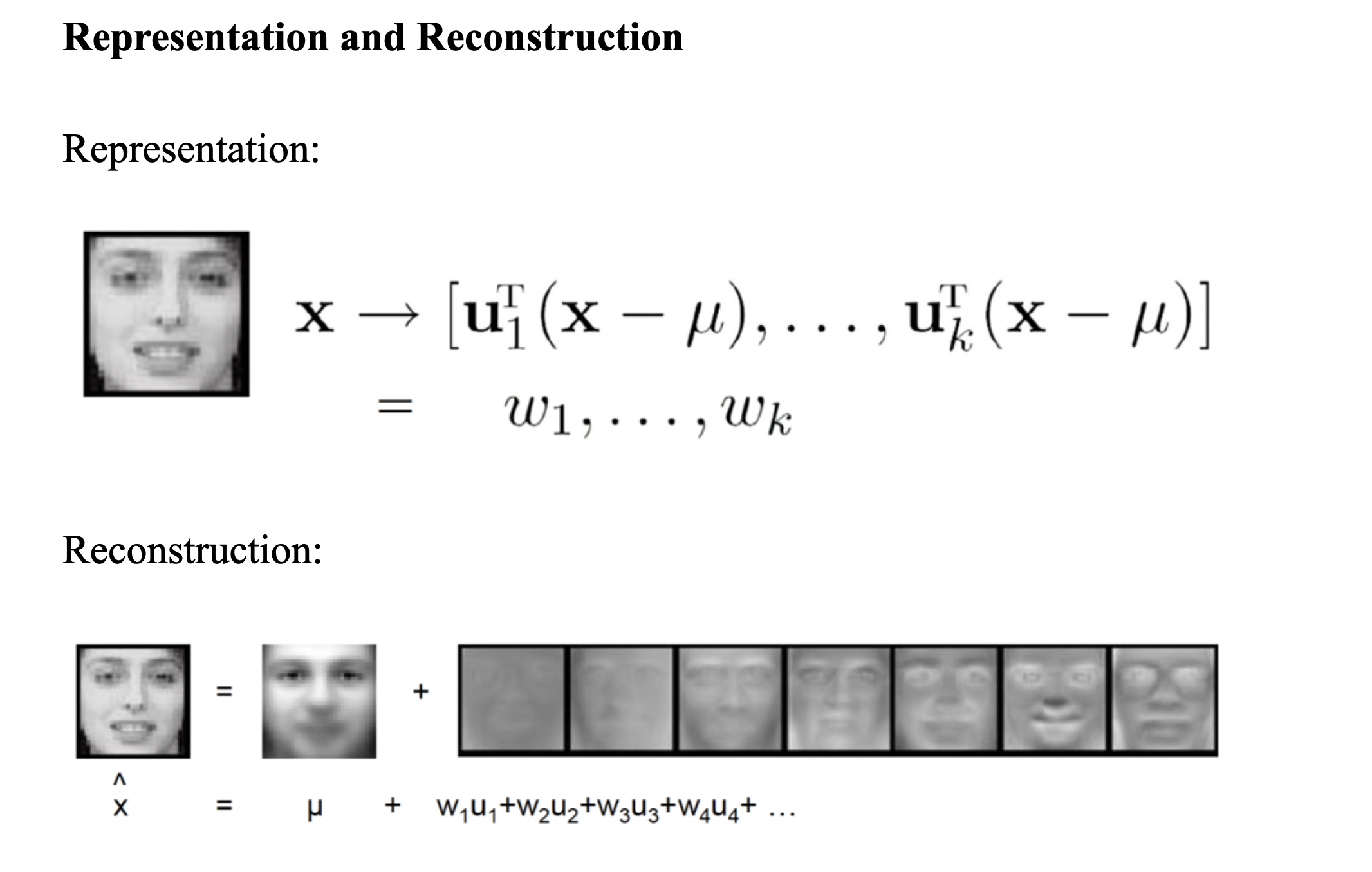
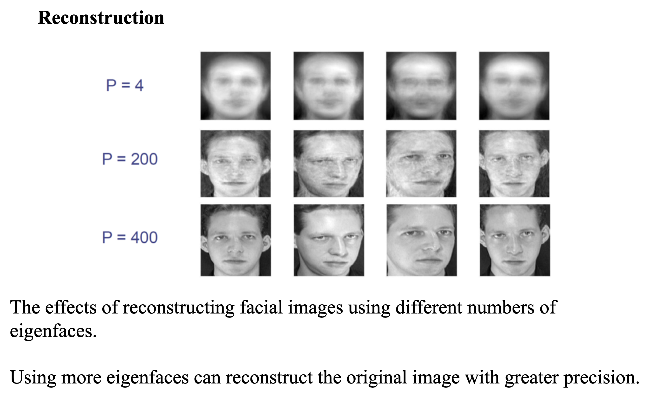
PCA Applications

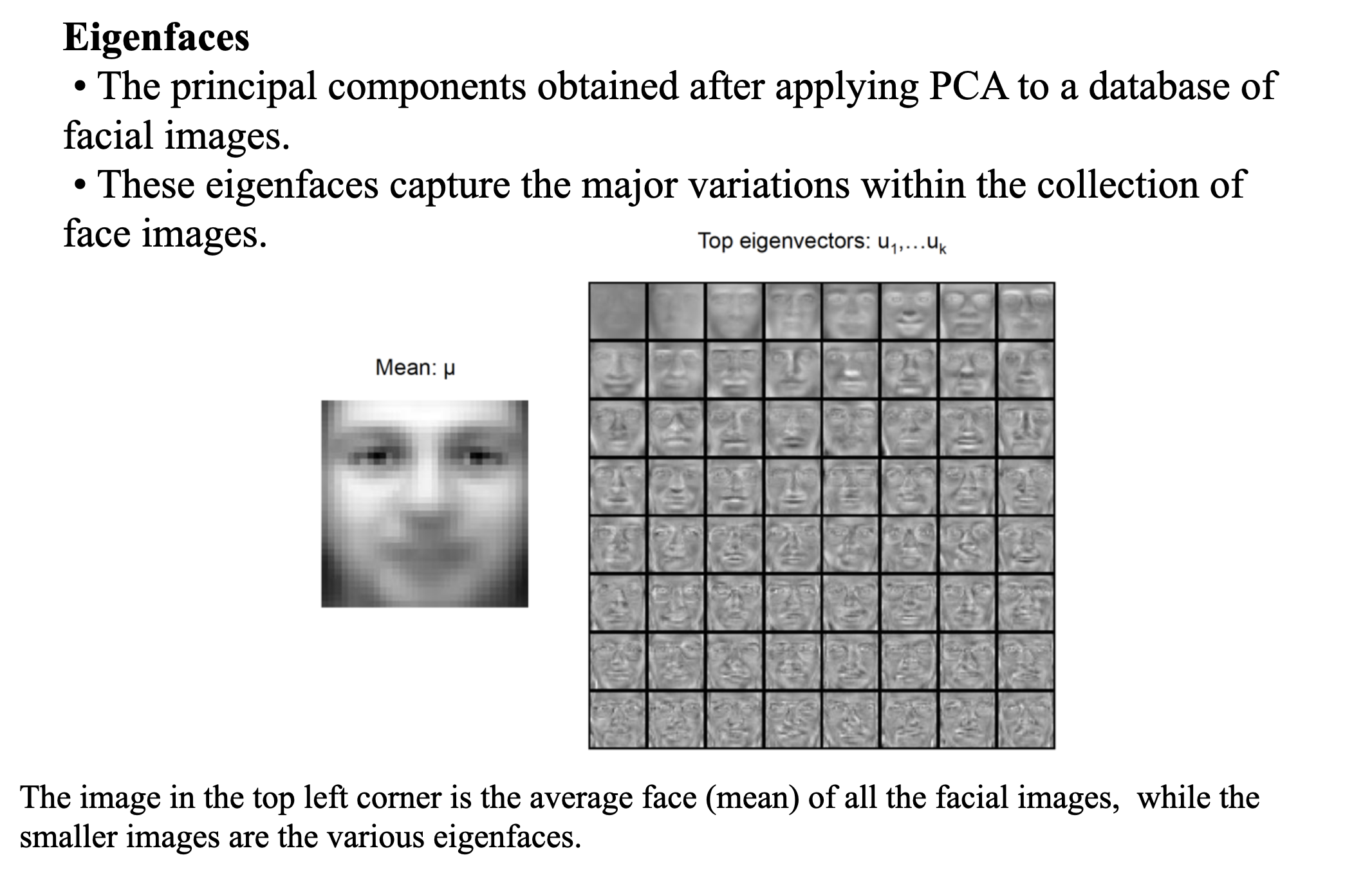
Clustering

Clustering: Divide a set of objects (e.g. data points) into a small number of disjoint groups such that objects in the same group are close together, and objects in different groups are far apart.

Organizing data into clusters such that there is
- high intra-cluster similarity
- low inter-cluster similarity
Informally, finding natural groupings among objects. A technique to divide a collection of objects (data points) into distinct groups where:
- Objects within the same group are similar (high intra-cluster similarity)
- Objects from different groups are dissimilar (low inter-cluster similarity)

Key Characteristics:

Unsupervised learning - No predefined labels
Discovers natural groupings in data
Grouping based on similarity/distance metrics

Why Use Clustering?

Purpose	Example Applications
Data Organization	Document categorization, Customer segmentation
Pattern Discovery	Fraud detection, Anomaly identification
Knowledge Extraction	Market research, Biological data analysis
Preprocessing Step	Image compression, Dimensionality reduction

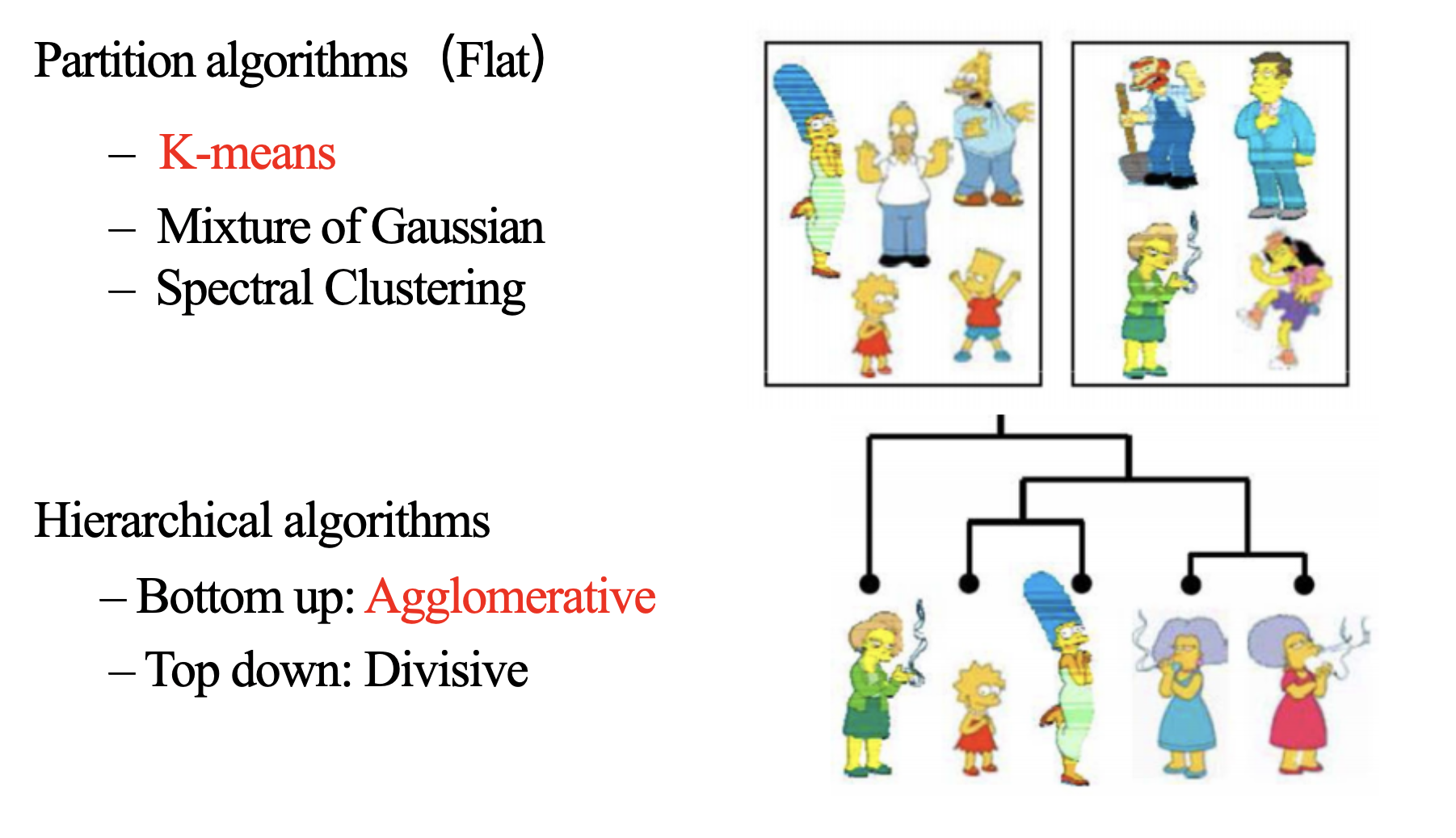
Clustering Algorithms

K-Means Clustering

How k-means clustering works?

We are given a data set of items with certain features and values for these features like a vector. The task is to categorize those items into groups. To achieve this we will use the K-means algorithm. 'K' in the name of the algorithm represents the number of groups/clusters we want to classify our items into. The algorithm will categorize the items into k groups or clusters of similarity. To calculate that similarity we will use the Euclidean distance as a measurement. The algorithm works as follows:

First we randomly initialize k points called means or cluster centroids. We categorize each item to its closest mean and we update the mean's coordinates, which are the averages of the items categorized in that cluster so far.

We repeat the process for a given number of iterations and at the end, we have our clusters. The "points" mentioned above are called means because they are the mean values of the items categorized in them. To initialize these means, we have a lot of options. An intuitive method is to initialize the means at random items in the data set. Another method is to initialize the means at random values between the boundaries of the data set. For example for a feature x the items have values in [0,3] we will initialize the means with values for x at [0,3].

Step Wise

Assignment Step: Assign Points to Nearest Centroid
- Metric: Euclidean distance (default) calculates proximity between a point $x_i$ $x_{i}$ and centroid $μ_k$ $μ_{k}$ :
  - $D(\mathbf{x}_i, \boldsymbol{\mu}_k) = \sqrt{\sum_{j=1}^d (x_{ij} - \mu_{kj})^2}$
- Rule: Each point joins the cluster whose centroid is closest.
- Why: Minimizes intra-cluster distances, ensuring tight groupings.
Update Step: Recompute Centroids
- Action: Centroids shift to the mean of their assigned points:
- Effect: Centroids move toward the densest region of their cluster.
- Why? Averages reduce WCSS (Within-Cluster Sum of Squares), the algorithm’s optimization target:
Convergence: When Does It Stop?
- The algorithm terminates when:
- No reassignments: Points stay in the same clusters.
- Centroid stability: Movement falls below a threshold
- Max iterations reached (user-defined safeguard).
Why Finite Steps?
- WCSS decreases monotonically.
- Finite data points → finite possible assignments.

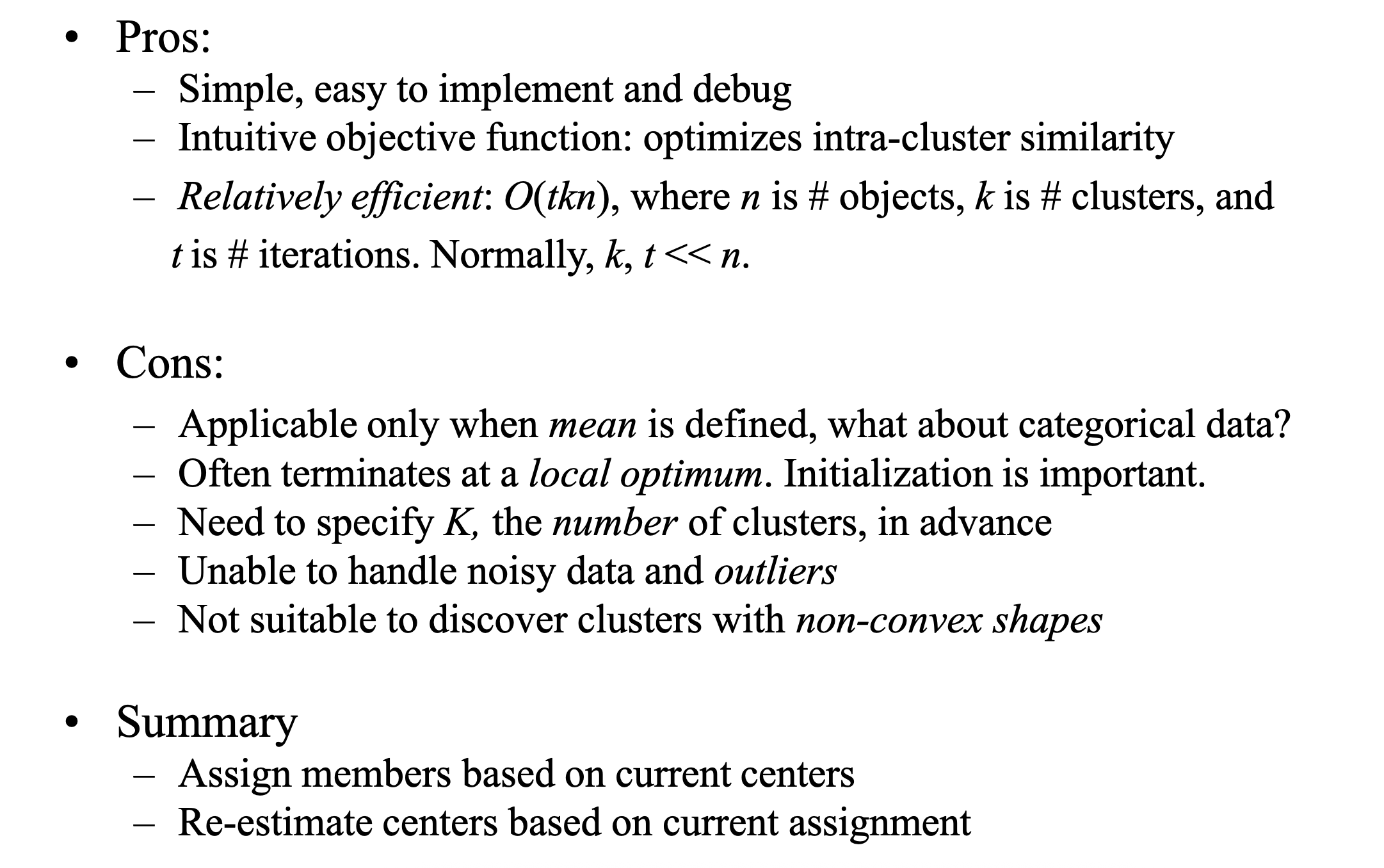
Properties of K-means

K-means is a popular clustering algorithm with several important properties:

Guaranteed to Converge in a Finite Number of Iterations
- K-means will always converge to a local minimum in a finite number of iterations because:
- Finite Possible Clusterings: There are a finite number of possible cluster assignments (though exponentially large).
- Monotonic Improvement: Each iteration reduces the objective function (sum of squared distances from points to their cluster centers) or leaves it unchanged.
- No Cycles: Since the objective function strictly decreases or stays the same, the algorithm cannot enter an infinite loop.
- Note: The convergence is to a local optimum, not necessarily the global optimum.
Running Time Per Iteration
- K-means iterates between two main steps, each with a well-defined computational cost:
- Step 1: Assign Data Points to Closest Cluster Center
  - For each of the N data points, compute the distance to all K cluster centers.
  - Time complexity: O(KN), since each of the N points requires K distance calculations.
- Step 2: Update Cluster Centers to the Average of Assigned Points
  - For each of the K clusters, compute the mean of all points assigned to it.
  - This involves summing O(N) points (in the worst case, all points could belong to one cluster, though typically it’s O(N/K) per cluster).
  - Time complexity: O(N), since each of the N points is added to one cluster’s sum.
- Total Time per Iteration: O(KN)+O(N)=O(KN).
  - Typically, K≪N, so the assignment step dominates.

Additional Notes:

The number of iterations required for convergence depends on the data and initialization, but it is often small in practice (e.g., tens of iterations).
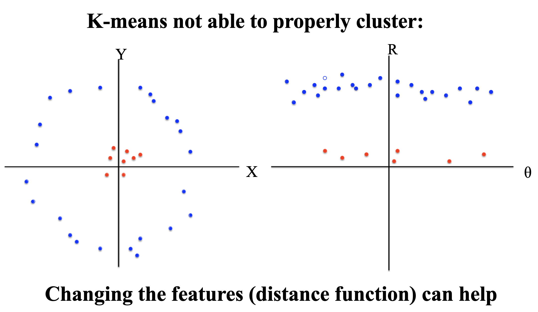
The algorithm is efficient for low-dimensional data but can suffer in high dimensions due to the curse of dimensionality (distance computations become less meaningful).
Sensitive to initial cluster centers (common workarounds: multiple random restarts or k-means++ initialization).

Initialization Methods to Improve K-means

To avoid bad local optima, several initialization schemes exist:

Random Initialization (Basic)
- Randomly pick K data points as initial centers.
- Problem: Highly unstable; may require multiple restarts.
Variance-Based Splitting (Old Approach)
- Start with one cluster (mean = global centroid).
- Iteratively split the cluster with the highest variance.
- Disadvantage: Computationally expensive, not commonly used now.
K-means++ (Best-Practice Initialization)
- A smarter way to choose initial centers to spread them out:
- First center: Randomly pick one data point.
- Next centers:
  - Compute distances $D(x)$ of each point to the nearest existing center.
  - Choose the next center with probability proportional to $D(x)^2$ (i.e., far from existing centers).
- Repeat until K centers are selected.

Advantages:

Reduces the risk of bad initialization.
Leads to faster convergence and better clustering.
Theoretically guarantees $O(logK)$ approximation to optimal clustering.

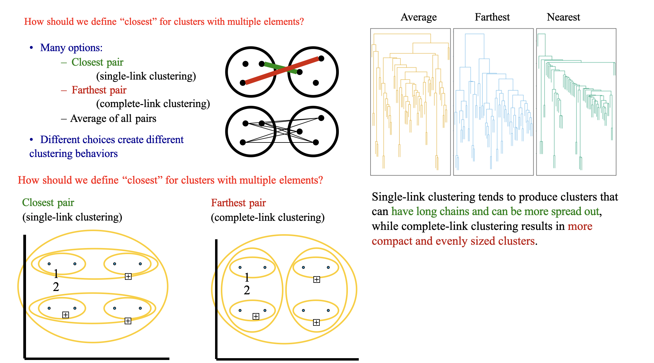
Hierarchical Agglomerative Clustering

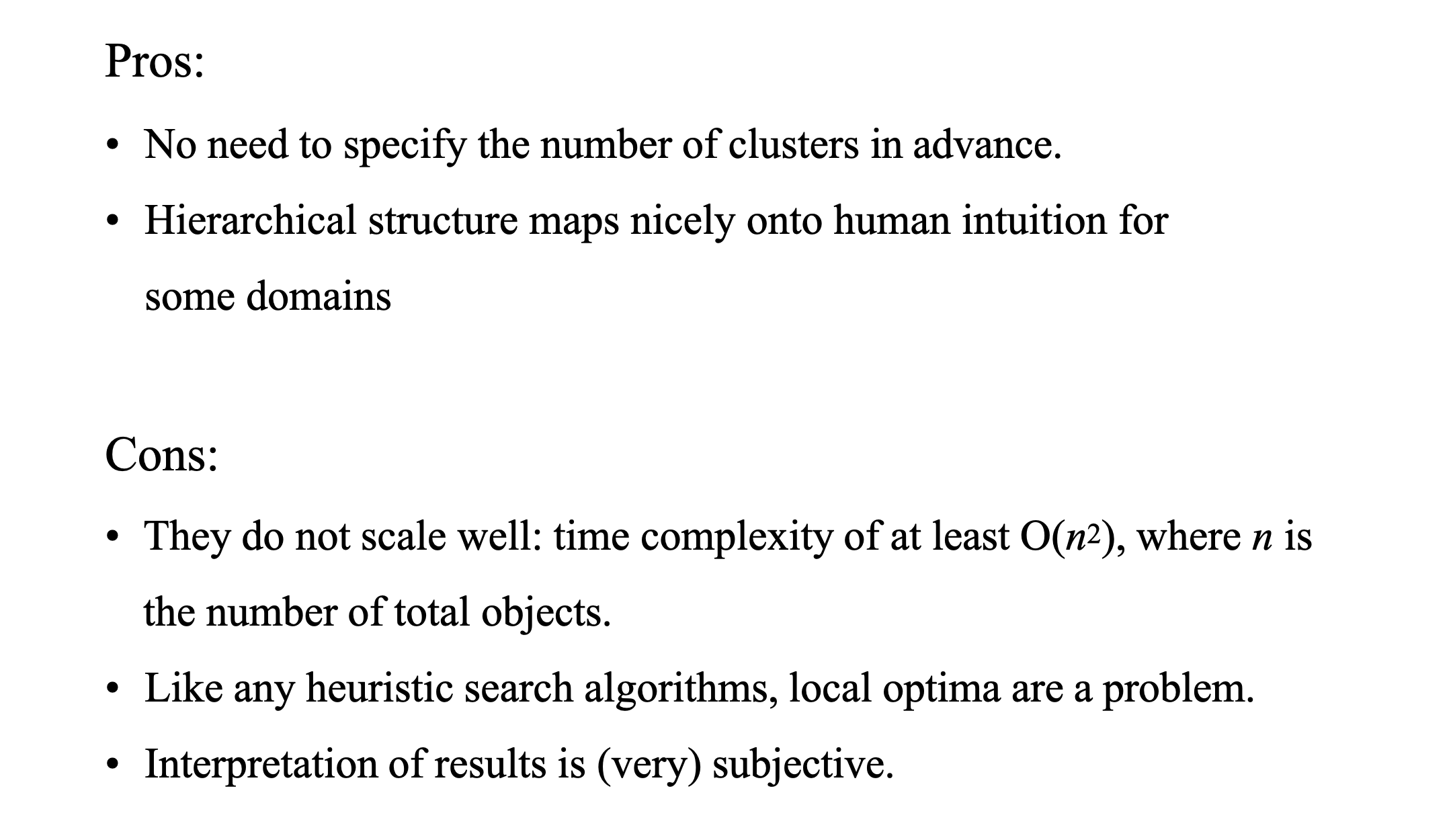
It is also known as the bottom-up approach or hierarchical agglomerative clustering (HAC). Unlike flat clustering hierarchical clustering provides a structured way to group data. This clustering algorithm does not require us to prespecify the number of clusters. Bottom-up algorithms treat each data as a singleton cluster at the outset and then successively agglomerate pairs of clusters until all clusters have been merged into a single cluster that contains all data.

Workflow for Hierarchical Agglomerative clustering

Start with individual points: Each data point is its own cluster. For example if you have 5 data points you start with 5 clusters each containing just one data point.
Calculate distances between clusters: Calculate the distance between every pair of clusters. Initially since each cluster has one point this is the distance between the two data points.
Merge the closest clusters: Identify the two clusters with the smallest distance and merge them into a single cluster.
Update distance matrix: After merging you now have one less cluster. Recalculate the distances between the new cluster and the remaining clusters.
Repeat steps 3 and 4: Keep merging the closest clusters and updating the distance matrix until you have only one cluster left.
Create a dendrogram: As the process continues you can visualize the merging of clusters using a tree-like diagram called a dendrogram. It shows the hierarchy of how clusters are merged.