Lesson 1.13: Decision Tree Learning

A tree-like model that illustrates series of events leading to certain decisions. Each node represents a test on an attribute and each branch is an outcome of that test.

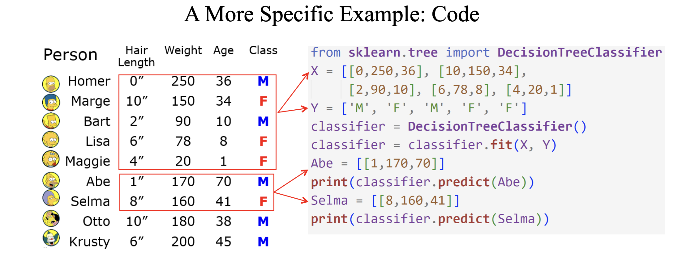
• We use labeled data to obtain a suitable decision tree for future predictions.
• We want a decision tree that works well on unseen data, while asking as few questions as possible.
• Basic step: choose an attribute and, based on its values, split the data into smaller sets.
• Recursively repeat this step until we can surely decide the label.

Pseudocode for making a decision tree

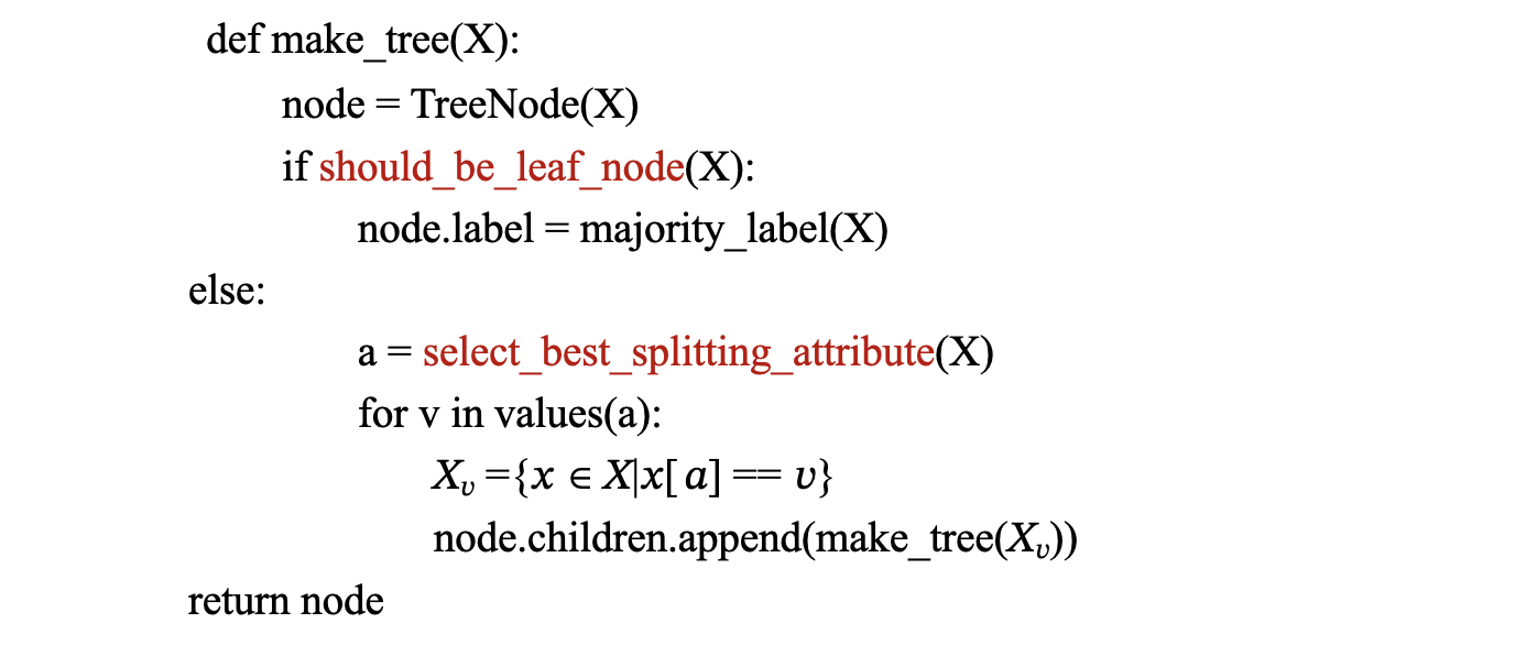
Decision Tree Learning Process

• Input: Labeled training data (features + target class)
• Goal: Build a tree that:
  • Generalizes well to unseen data
  • Makes decisions with minimal questions (shallow depth)
• Recursive Splitting:
  • Select best attribute at each node
  • Split data into subsets based on attribute values
  • Repeat until stopping criteria met

When to Create a Leaf Node?

A node becomes a leaf when:

• Pure node: All samples belong to one class (e.g., 100% "Yes" or 100% "No")
• No remaining features to split on
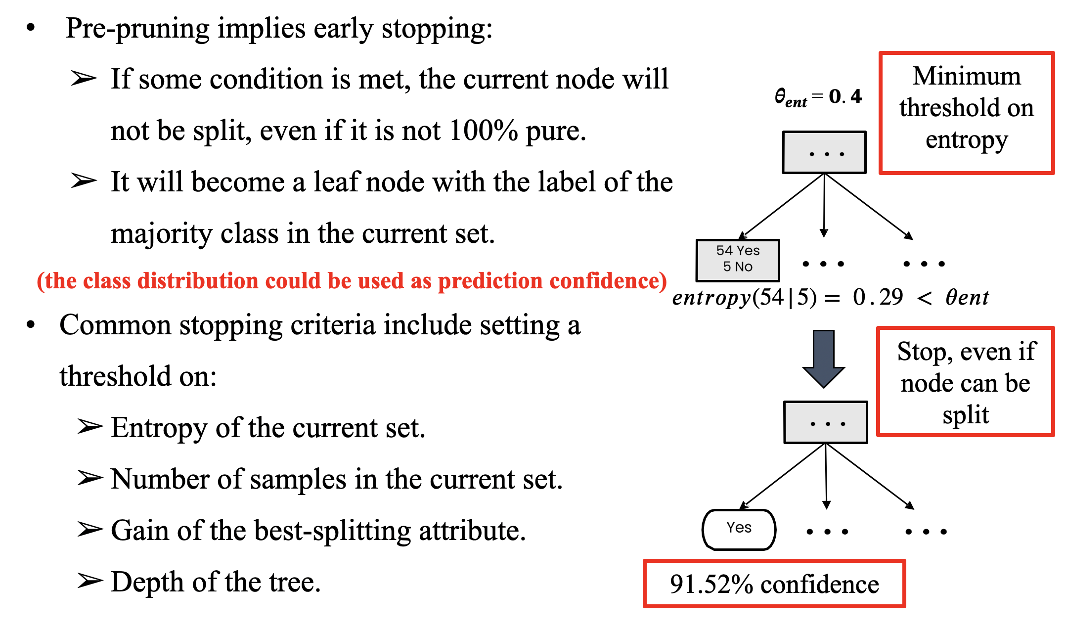
• Pre-pruning: Early stopping if split doesn't improve purity significantly

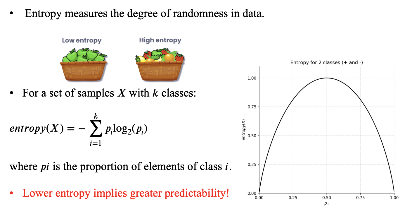
Entropy

Entropy measures the uncertainty or randomness in a dataset. It quantifies how "mixed" the class labels are in a given subset of data.

Information Gain

Information Gain (IG) measures how much an attribute reduces uncertainty (entropy) about the class when splitting a dataset. It helps select the best attribute for decision tree nodes.

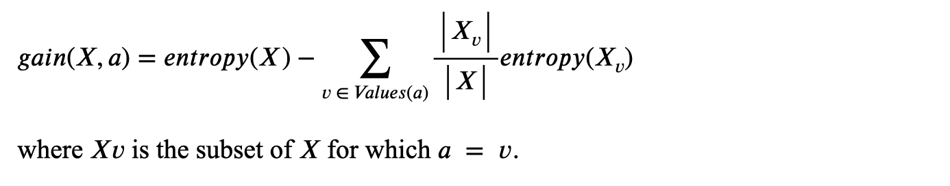
• For attribute A and dataset S:
• $\text{IG}(S, A) = H(S) - \sum_{v \in \text{Values}(A)} \frac{|S_v|}{|S|} H(S_v)$
• Where:
  • $H(S)$: Entropy of the original set $S$
  • $S_v$ : Subset of $S$ where attribute $A$ has value $v$
  • $\frac{|S_v|}{|S|}$ : Proportion of samples in subset $S_v$
• Goal: Maximize IG → Choose the attribute that most reduces entropy after splitting.

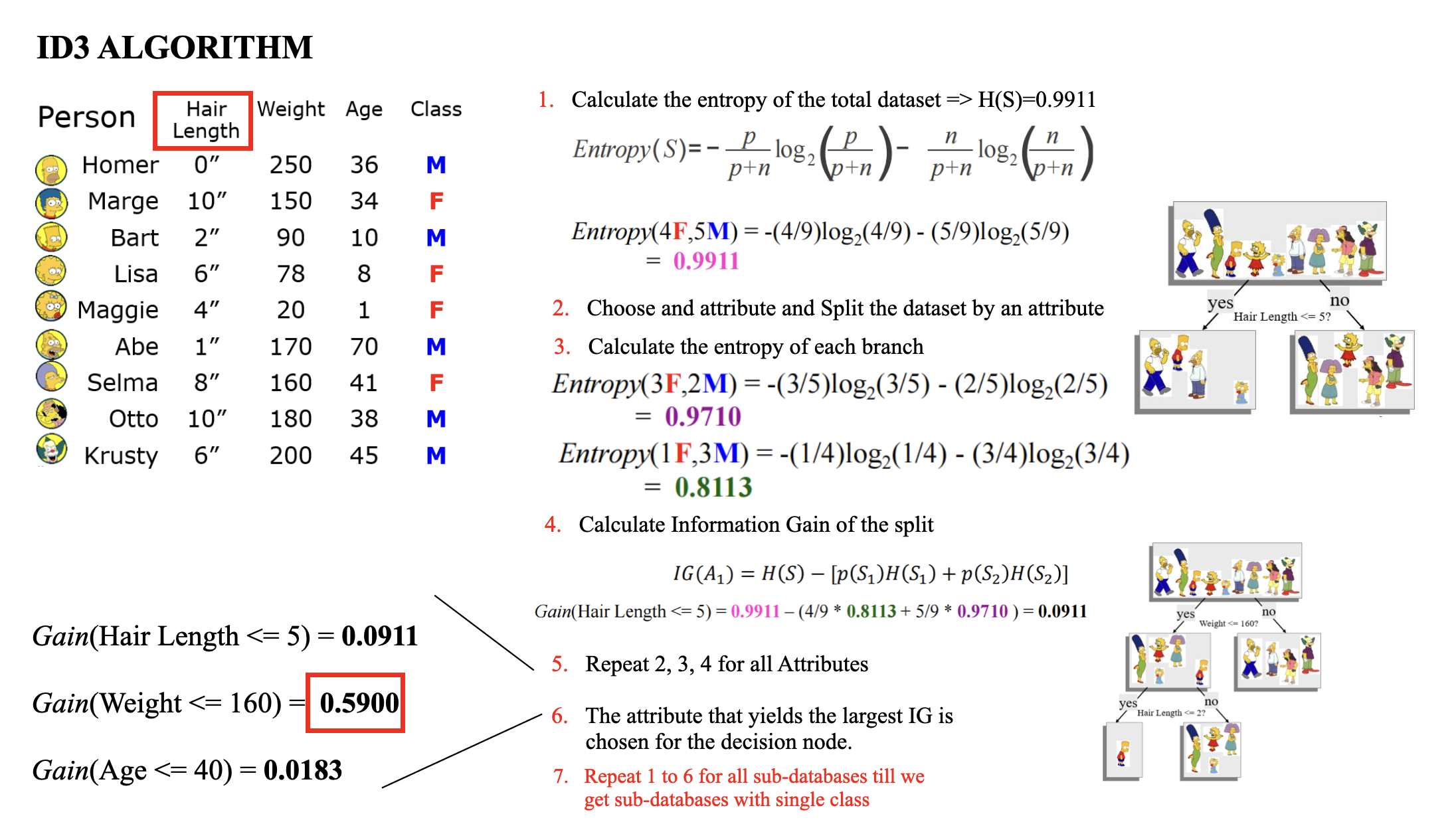
Step-by-Step Example

Dataset: Weather Conditions → Play Tennis?

Target: Predict "Play Tennis?" (Yes/No)

Information Gain Calculation in Decision Trees

Step 1: Calculate Original Entropy $H(S)$

Dataset Statistics:

• Total samples: 8
• Class distribution:
  • "Yes" (Play Tennis): 5
  • "No" (Don't Play): 3

Entropy Formula: $H(S) = -\left( p_{\text{Yes}} \log_2(p_{\text{Yes}}) + p_{\text{No}} \log_2(p_{\text{No}}) \right)$

Calculation: $H(S) = -\left( \frac{5}{8} \log_2\left(\frac{5}{8}\right) + \frac{3}{8} \log_2\left(\frac{3}{8}\right) \right) \approx 0.954 \text{ bits}$

Step 2: Calculate Entropy After Splitting on "Outlook"

Attribute Values:

• Sunny (3 samples)
• Overcast (2 samples)
• Rainy (3 samples)

a) Sunny Subset ($S_{\text{Sunny}}$)

• Samples: 3 "No", 0 "Yes" $H(S_{\text{Sunny}}) = 0 \text{ bits}$

b) Overcast Subset ($S_{\text{Overcast}}$)

• Samples: 2 "Yes", 0 "No" $H(S_{\text{Overcast}}) = 0 \text{ bits}$

c) Rainy Subset ($S_{\text{Rainy}}$)

• Samples: 2 "Yes", 1 "No" $H(S_{\text{Rainy}}) = -\left( \frac{2}{3} \log_2\left(\frac{2}{3}\right) + \frac{1}{3} \log_2\left(\frac{1}{3}\right) \right) \approx 0.918 \text{ bits}$

Weighted Average Entropy: $H(S|\text{Outlook}) = \left( \frac{3}{8} \times 0 + \frac{2}{8} \times 0 + \frac{3}{8} \times 0.918 \right) \approx 0.344 \text{ bits}$

Step 3: Compute Information Gain for "Outlook"

Information Gain Formula: $\text{IG}(S, \text{Outlook}) = H(S) - H(S|\text{Outlook})$

Calculation: $\text{IG}(S, \text{Outlook}) = 0.954 - 0.344 = 0.610 \text{ bits}$

Comparison with Other Attributes

Key Takeaways

1. Higher IG means better attribute for splitting
2. "Outlook" provides the most information about the target variable
3. The calculation follows:
   • Compute original entropy
   • Calculate weighted entropy after split
   • Subtract to get information gain

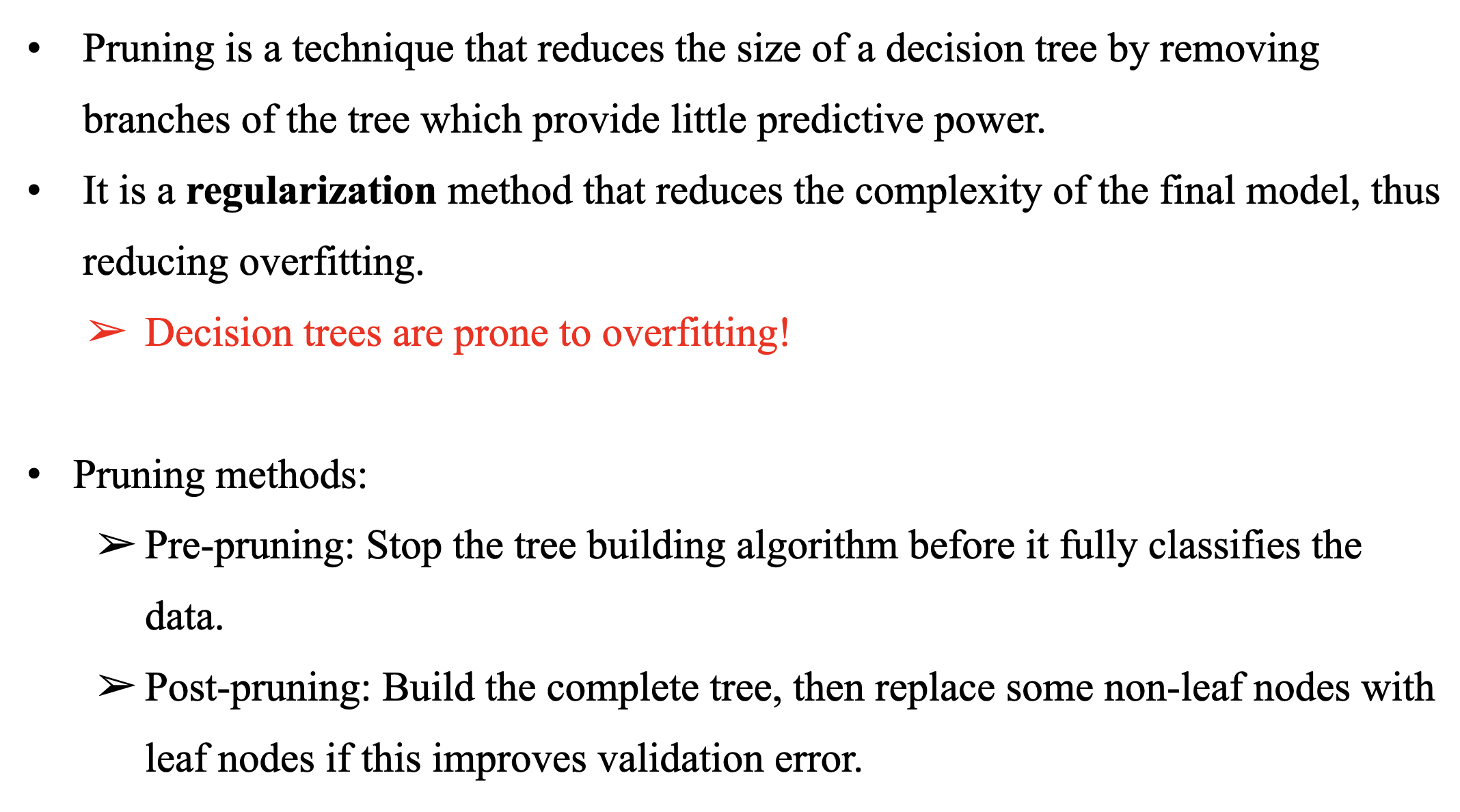
Pruning

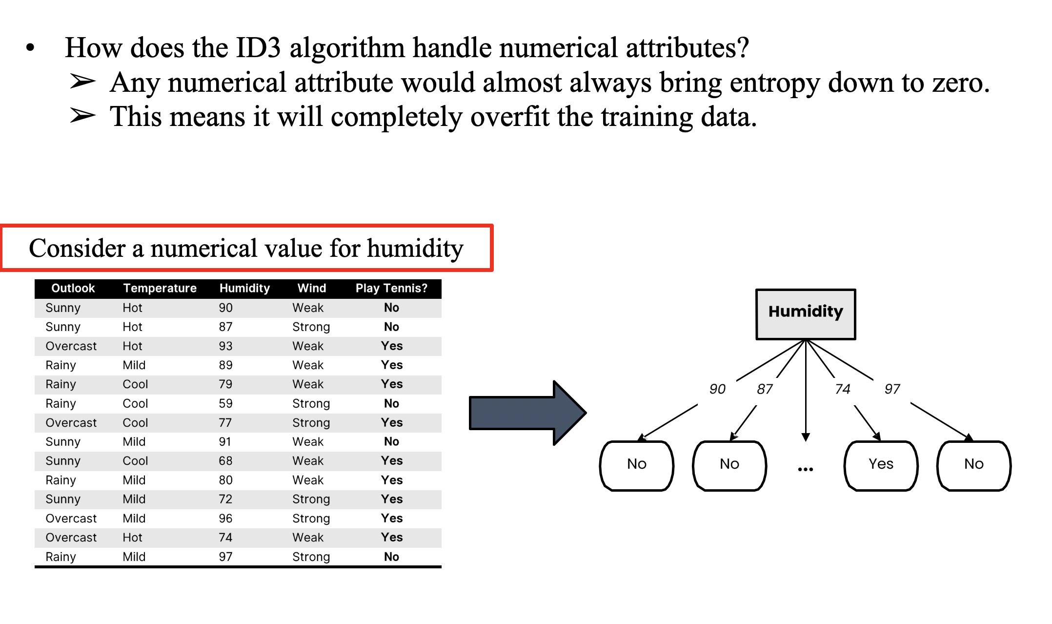
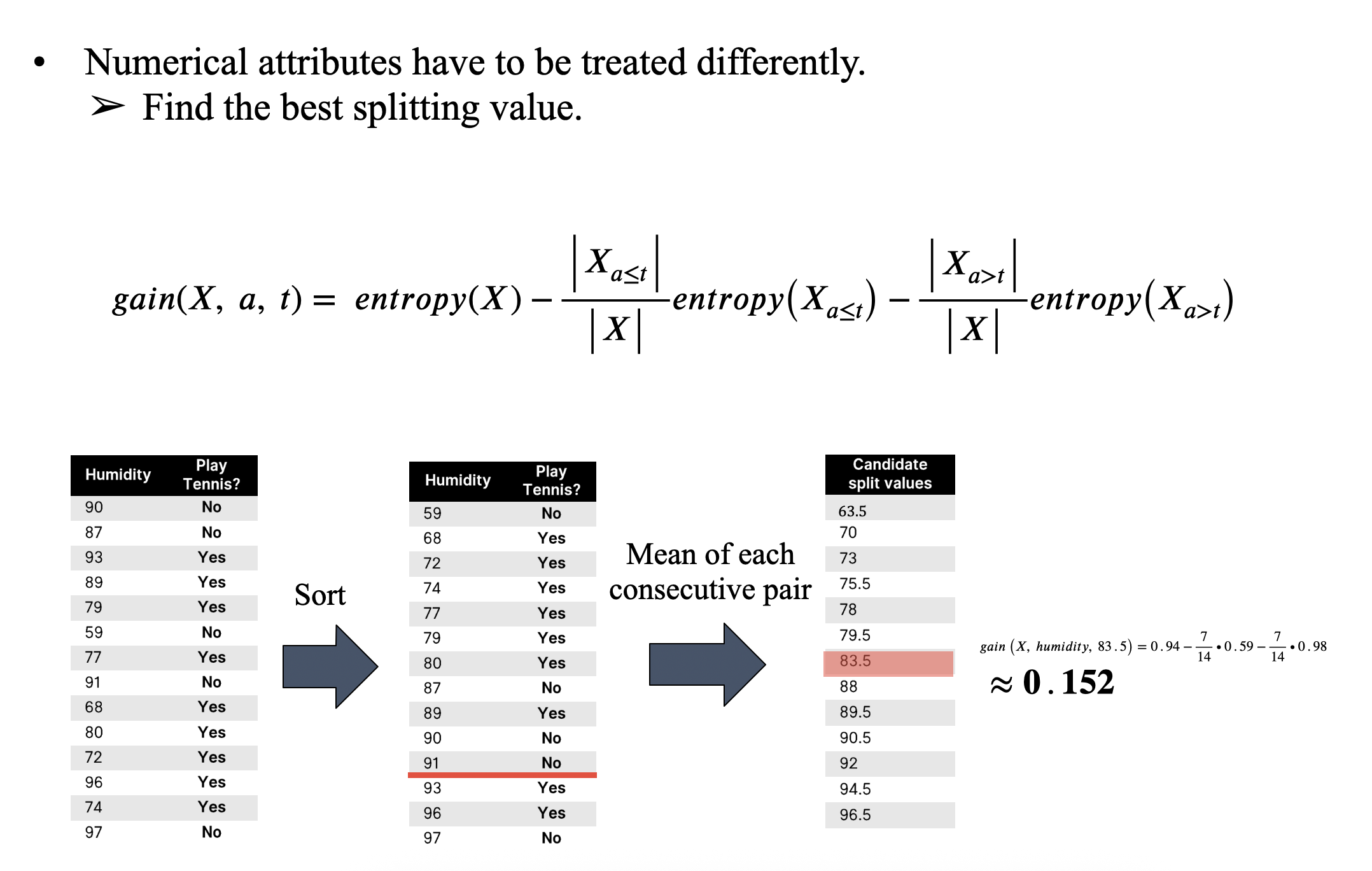
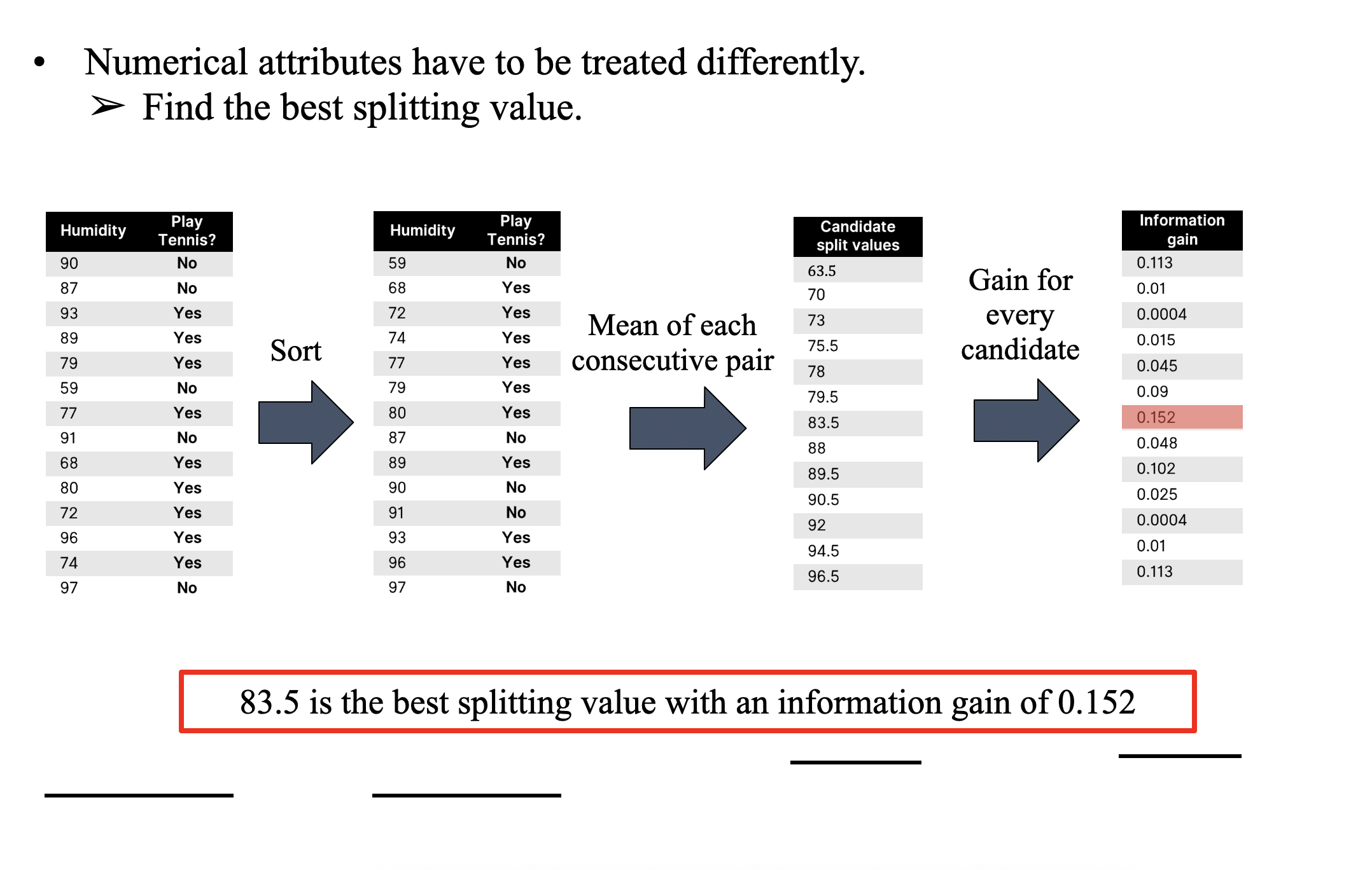
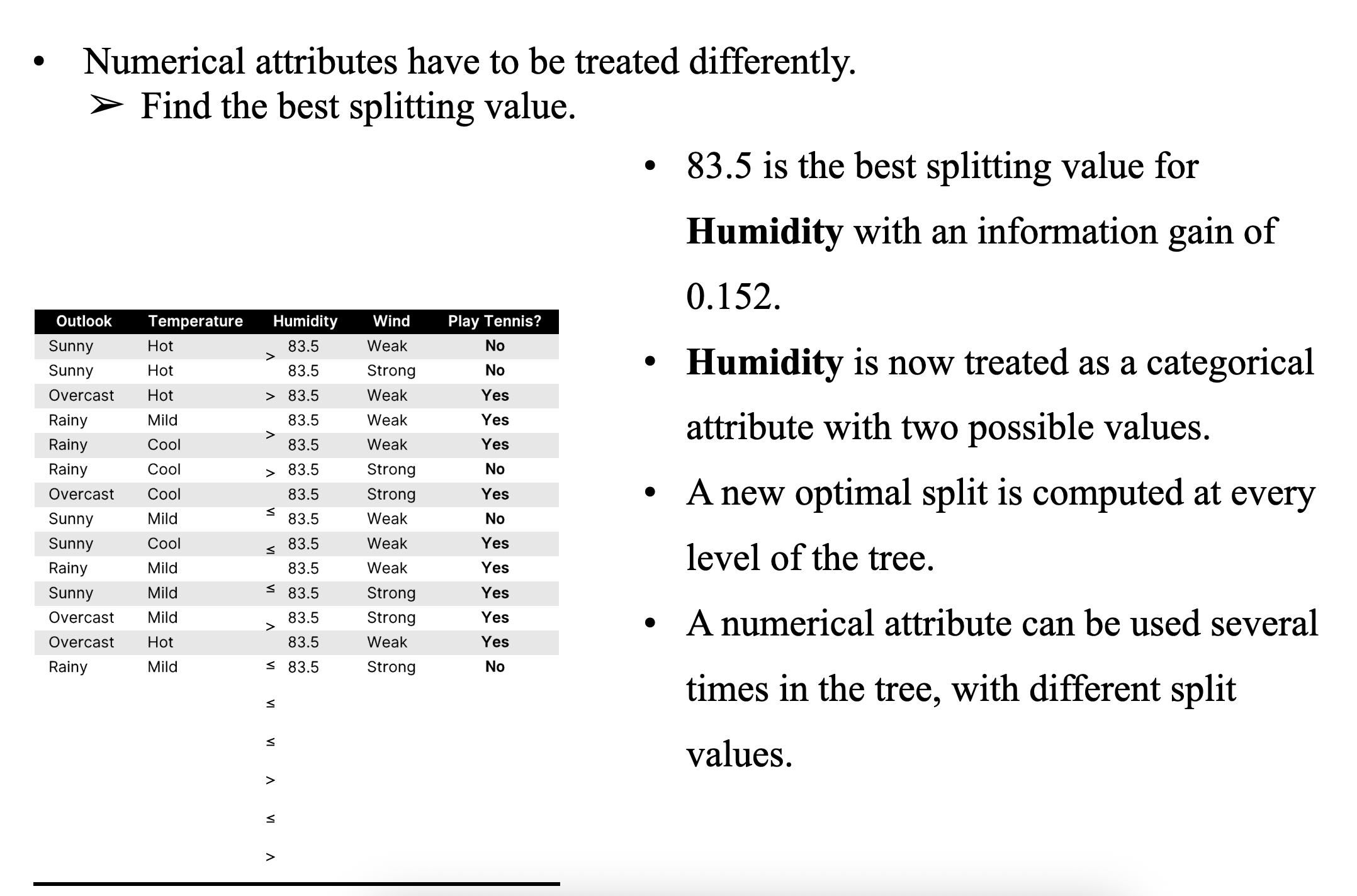
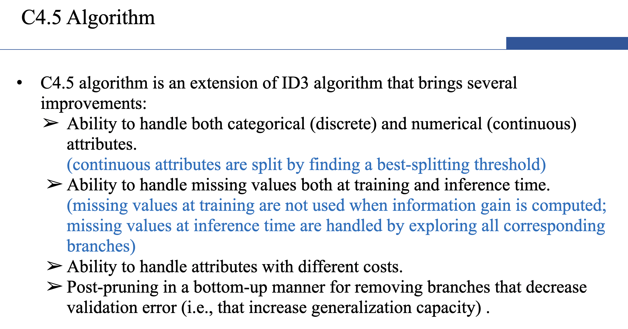
Handling Numerical Attributes

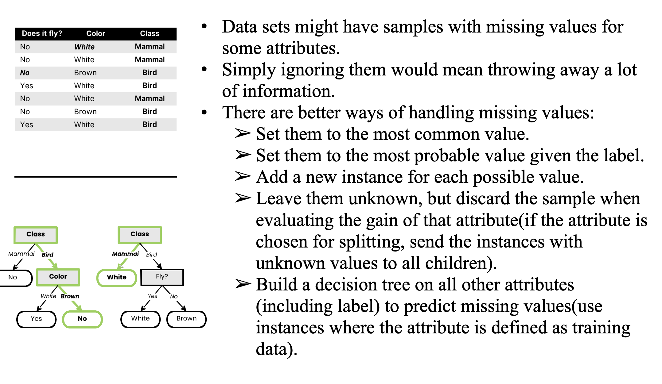
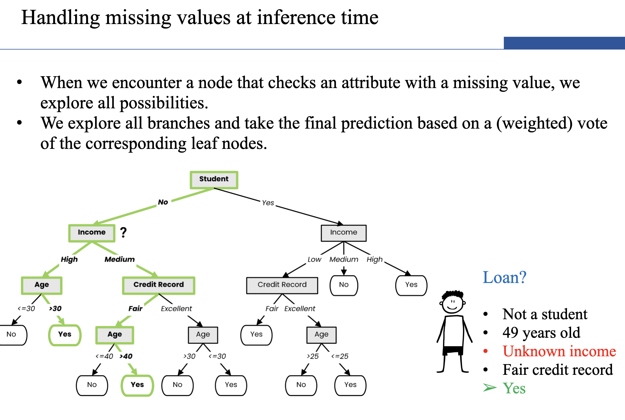
Handling Missing Attributes

Random Forests (Ensemble Learning With Decision Trees)

• Instead of building a single decision tree and use it to make predictions, build many slightly different trees and combine their predictions.
• We have a single data set, so how do we obtain slightly different trees?
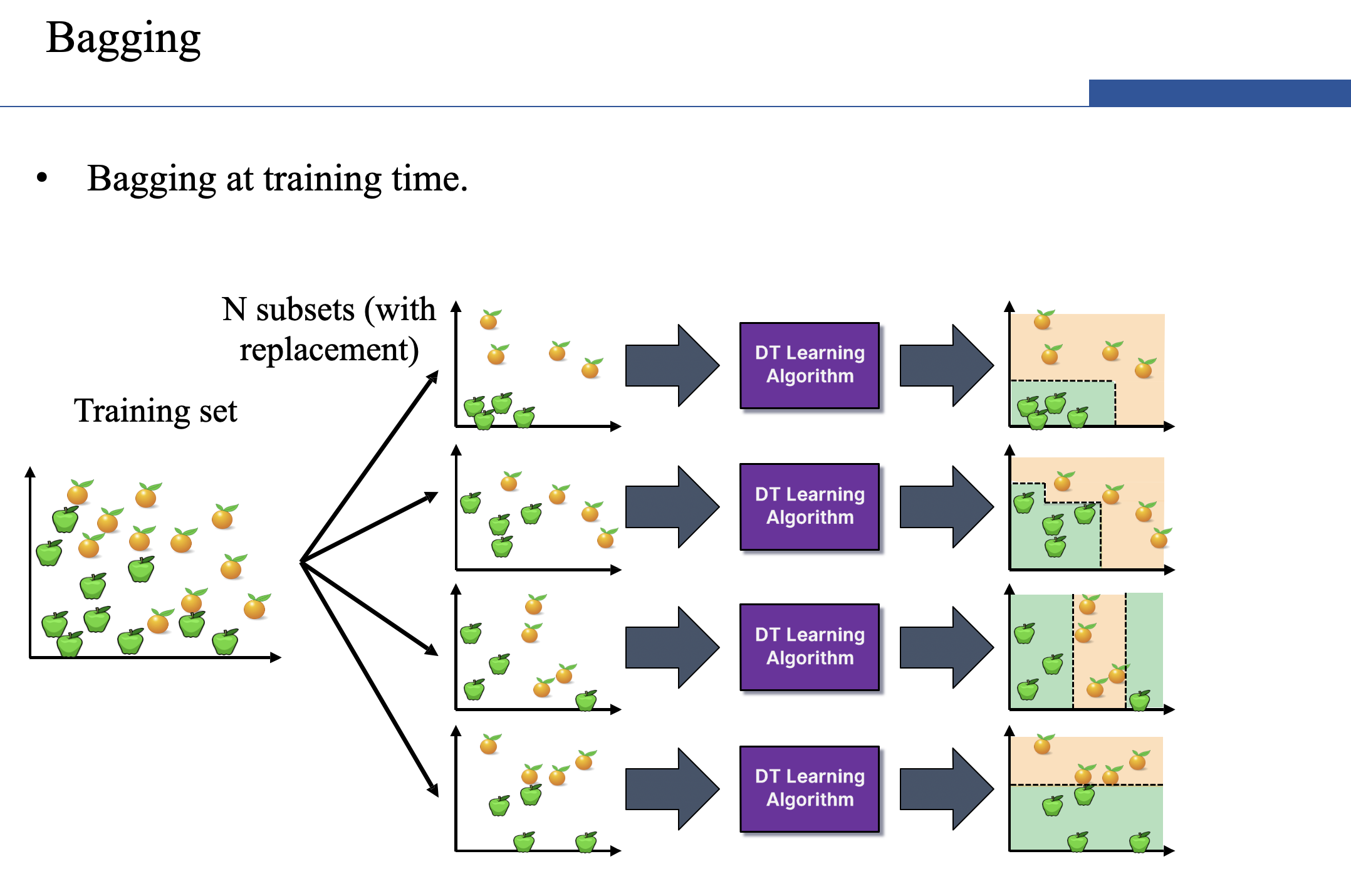
  1. Bagging (Bootstrap Aggregating):
     • Take random subsets of data from the training set to create N smaller data sets.
     • Fit a decision tree on each subset.
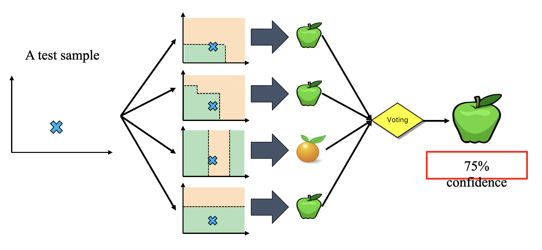
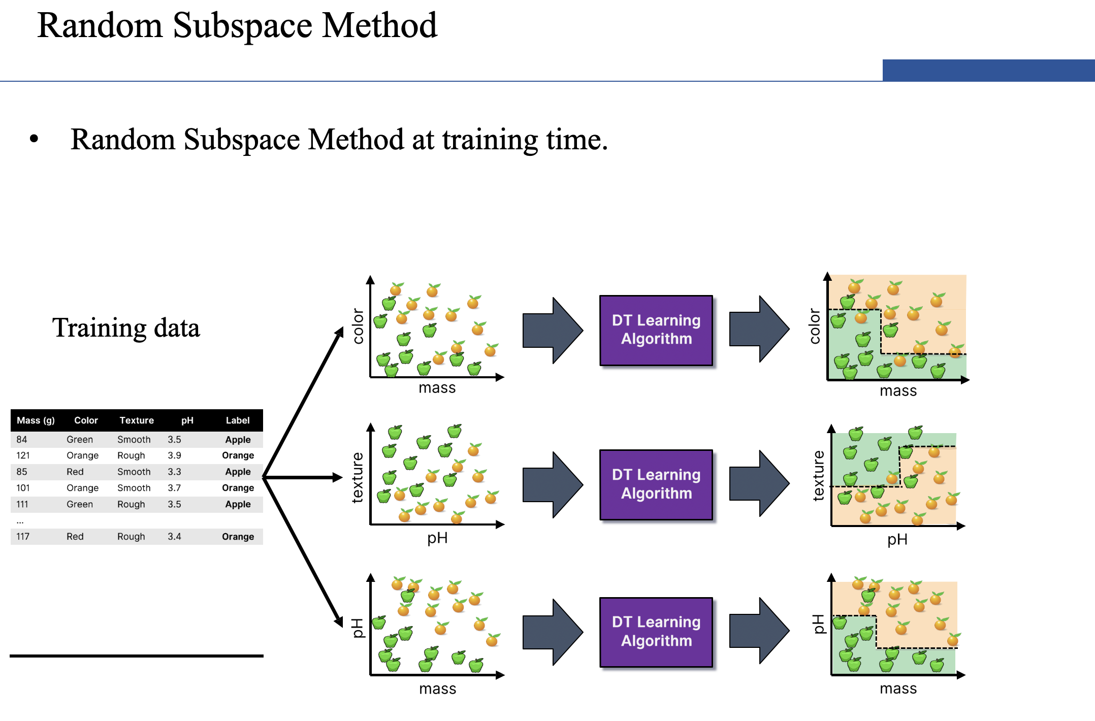
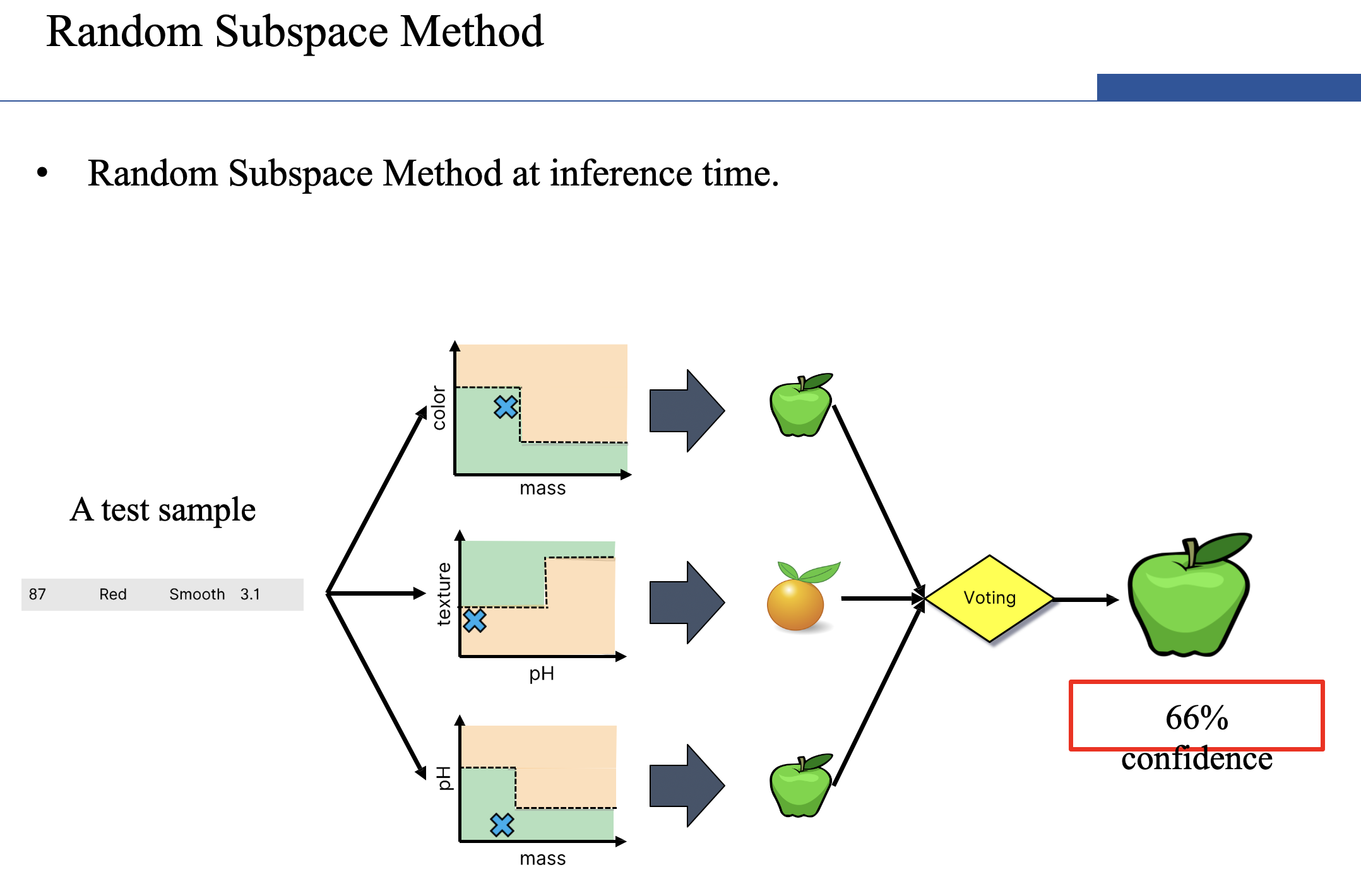
  2. Random Subspace Method (also known as Feature Bagging):
     • Fit N different decision trees by constraining each one to operate on a random subset of features.

Ensemble Learning

• Ensemble Learning:
  • Method that combines multiple learning algorithms to obtain performance improvements over its components.
• Random Forests are one of the most common examples of ensemble learning.
• Other commonly-used ensemble methods:
  • Bagging: multiple models on random subsets of data samples.
  • Random Subspace Method: multiple models on random subsets of features.
  • Boosting: train models iteratively, while making the current model focus on the mistakes of the previous ones by increasing the weight of misclassified samples.

Random Forests are an ensemble learning method that employ decision tree learning to build multiple trees through bagging and random subspace method. They rectify the overfitting problem of decision trees!