Lesson 1.9: Supervised Learning: K-Nearest Neighbours & Naive Bayes

K-Nearest Neighbours

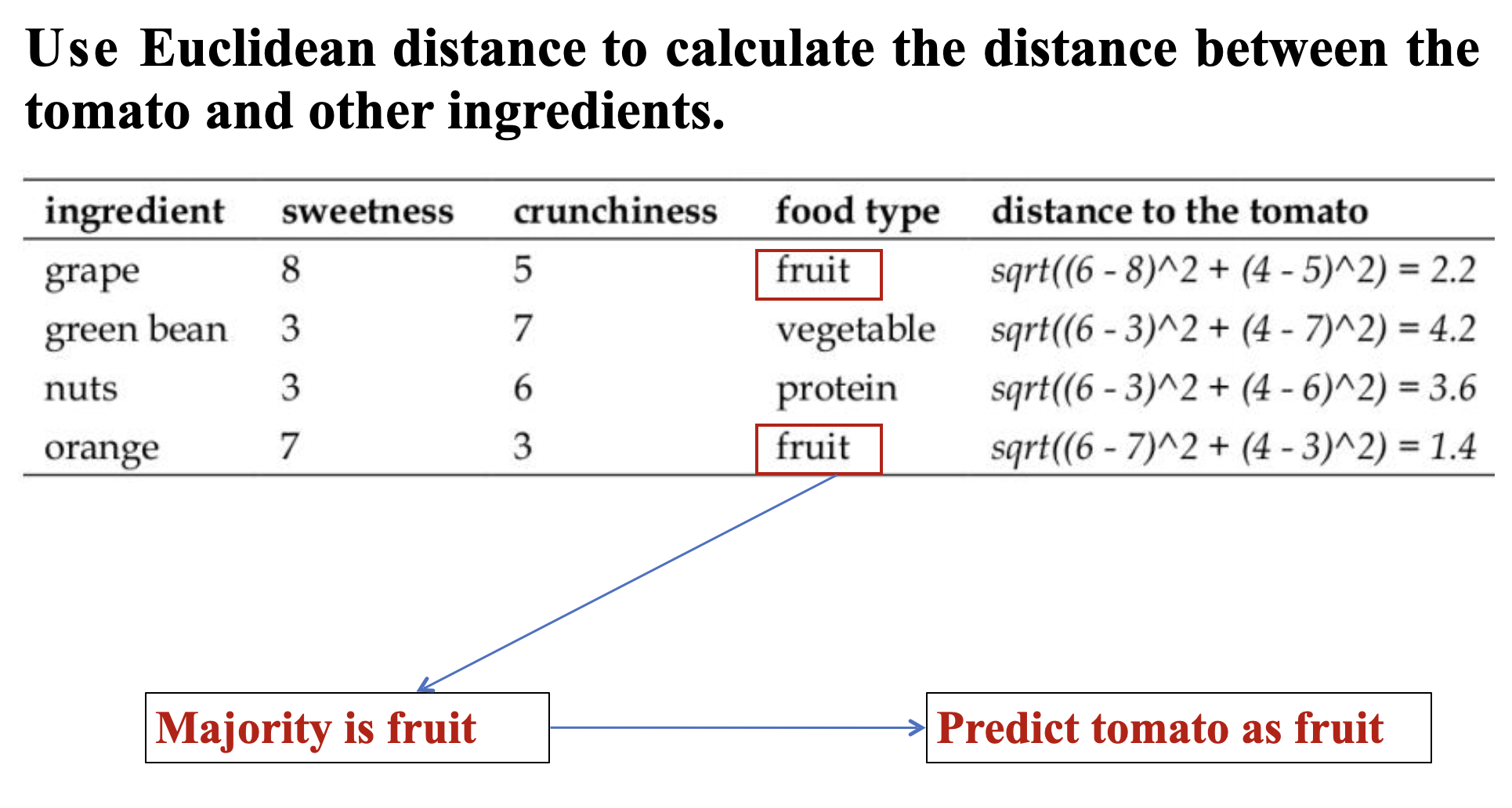
KNN is a simple yet powerful instance-based (or lazy learning) algorithm used for classification and regression. For classification, it assigns a class label to an unlabeled example based on the majority class among its $k$ closest neighbors in the training data.

Nearest Neighbor Classification

Classifies an unlabeled example by assigning it the class of the most similar labeled examples.
1-NN: The simplest case where k=1. The label is assigned based on the single closest neighbor.

K-Nearest Neighbors (KNN) Classification

Generalizes the idea by considering k closest neighbors.
The class label is determined by majority voting among the k neighbors.

Calculating Distance

KNN relies on distance metrics to determine similarity. Common distance measures include:

Manhattan Distance (L1 Norm)

$d(\mathbf{x}, \mathbf{y}) = \sum_{i=1}^{n} |x_i - y_i|$

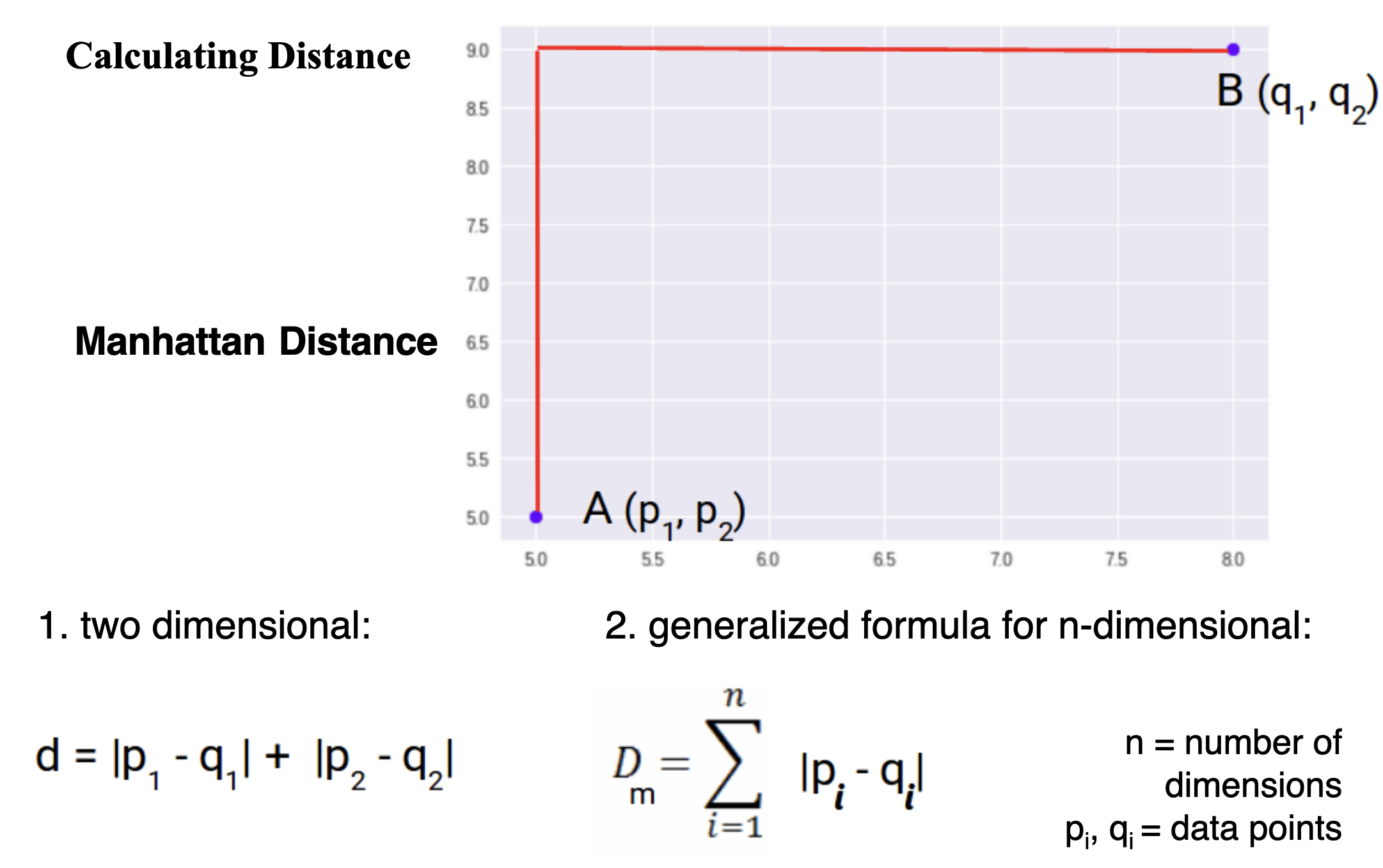
Sum of absolute differences between coordinates.

Euclidean Distance (L2 Norm)

$d(\mathbf{x}, \mathbf{y}) = \sqrt{\sum_{i=1}^{n} (x_i - y_i)^2}$

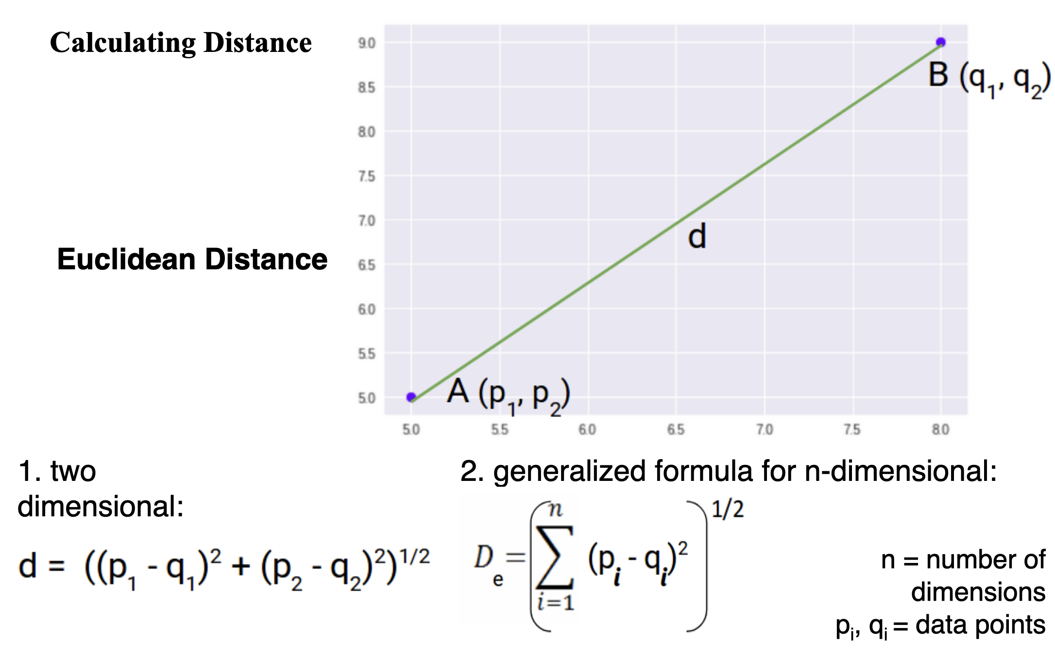
Straight-line distance between points in space.

Choosing the Right $k$

Small $k$ (e.g., $k = 1$ )

Highly sensitive to noise (overfitting).
Decision boundary is more complex.

Large $k$

Smoother decision boundaries (underfitting).
Computationally expensive.

Common Practices for Selecting $k:$

Typically set between 3 and 10.
A heuristic: $k \approx \sqrt{n}$ where $n$ is the number of training samples.
Deciding how many neighbors to use for KNN determines how well the mode will generalize to future data.
Choosing a large k reduces the impact or variance caused by noisy data, but can bias the learner such that it runs the risk of ignoring small, but important patterns.
In practice, choosing k depends on the difficulty of the concept to be learned and the number of records in the training data.
Typically, k is set somewhere between 3 and 10. One common practice is to set k equal to the square root of the number of training examples.
In the classifier, we might set k = 4, because there were 15 example ingredients in the training data and the square root of 15 is 3.87.

Min-Max Normalization

Since KNN is distance-based, features should be normalized to prevent bias from large-valued features. $X_{\text{norm}} = \frac{X - X_{\min}}{X_{\max} - X_{\min}}$

Scales all features to [0,1].
Ensures equal contribution from all features in distance calculation.
The traditional method of rescaling features for KNN is min-max normalization.
This process transforms a feature such that all of its values fall in a range between 0 and 1. The formula for normalizing a feature is as follows. Essentially, the formula subtracts the minimum of feature X from each value and divides by the range of X:
Normalized feature values can be interpreted as indicating how far, from 0 percent to 100 percent, the original value fell along the range between the original minimum and maximum.

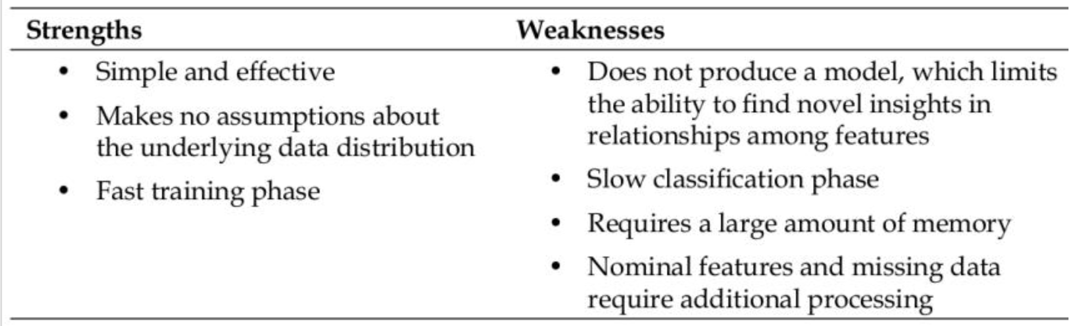
Lazy Learning (Instance-Based Learning)

No explicit training phase: Simply stores the training data ("rote learning").
Prediction phase is slower: Requires computing distances to all training points for each query.
Using the strict definition of learning, a lazy learner is not really learning anything.
Instead, it merely stores the training data in it. This allows the training phase to occur very rapidly, with a potential downside being that the process of making predictions tends to be relatively slow.
Due to the heavy reliance on the training instances, lazy learning is also known as instance-based learning or rote learning.
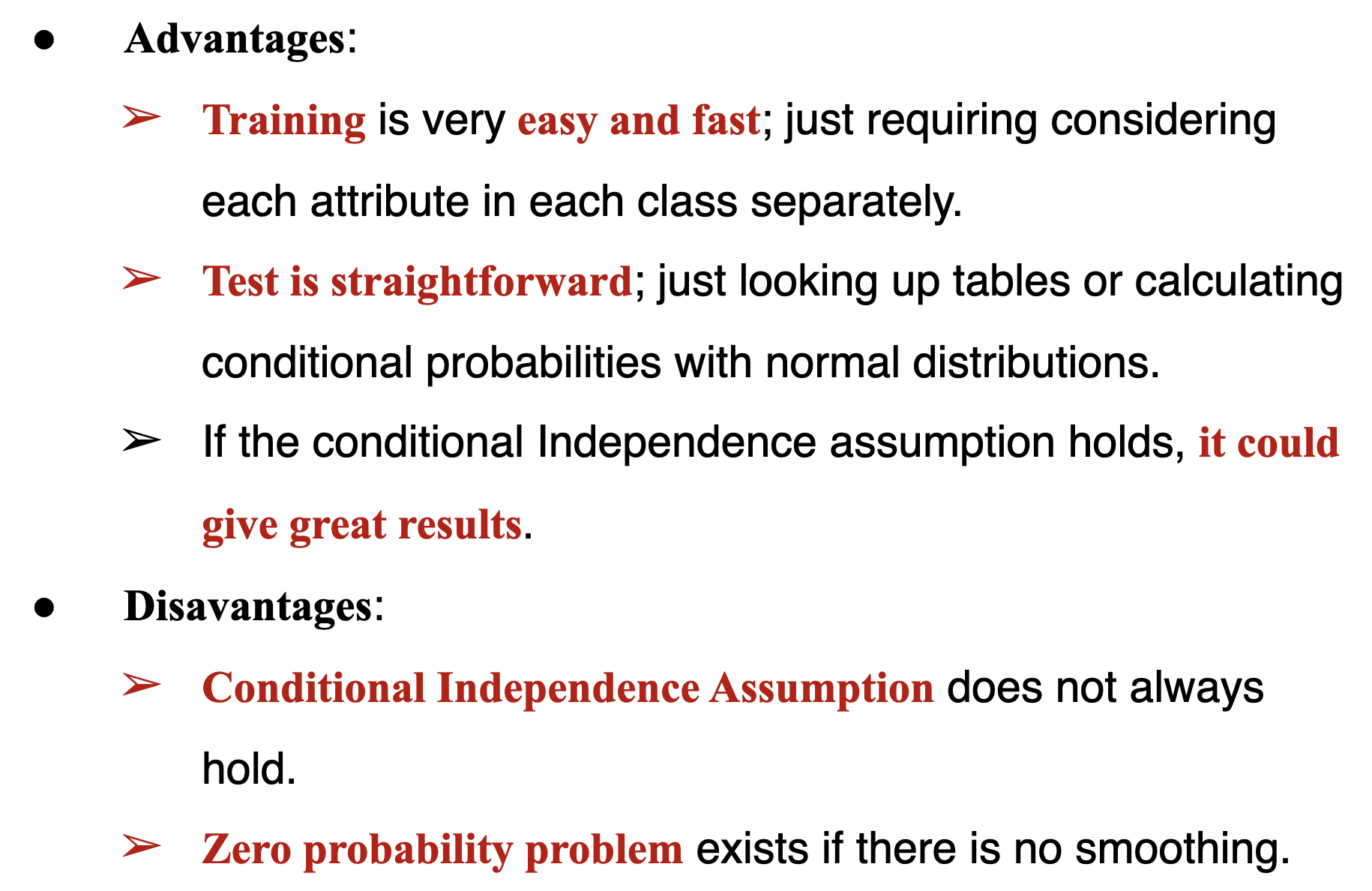
Advantages:
- Adapts immediately to new data.
- No assumptions about data distribution.
Disadvantages:
- Computationally expensive for large datasets.
- Sensitive to irrelevant/noisy features.

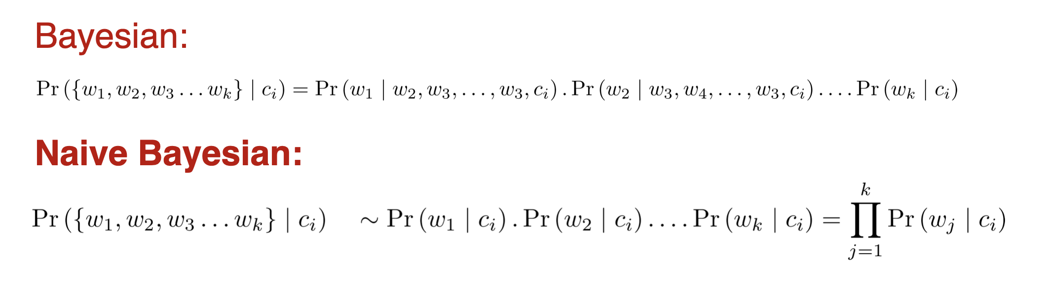
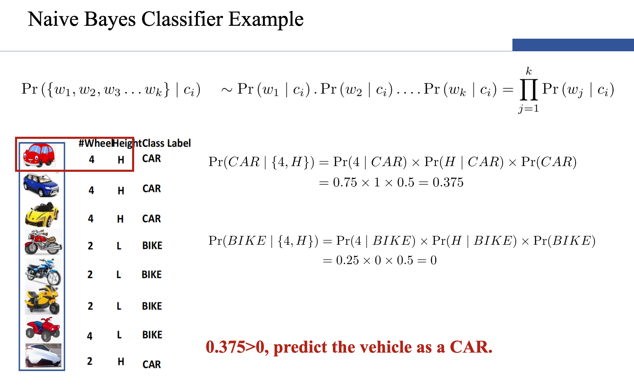
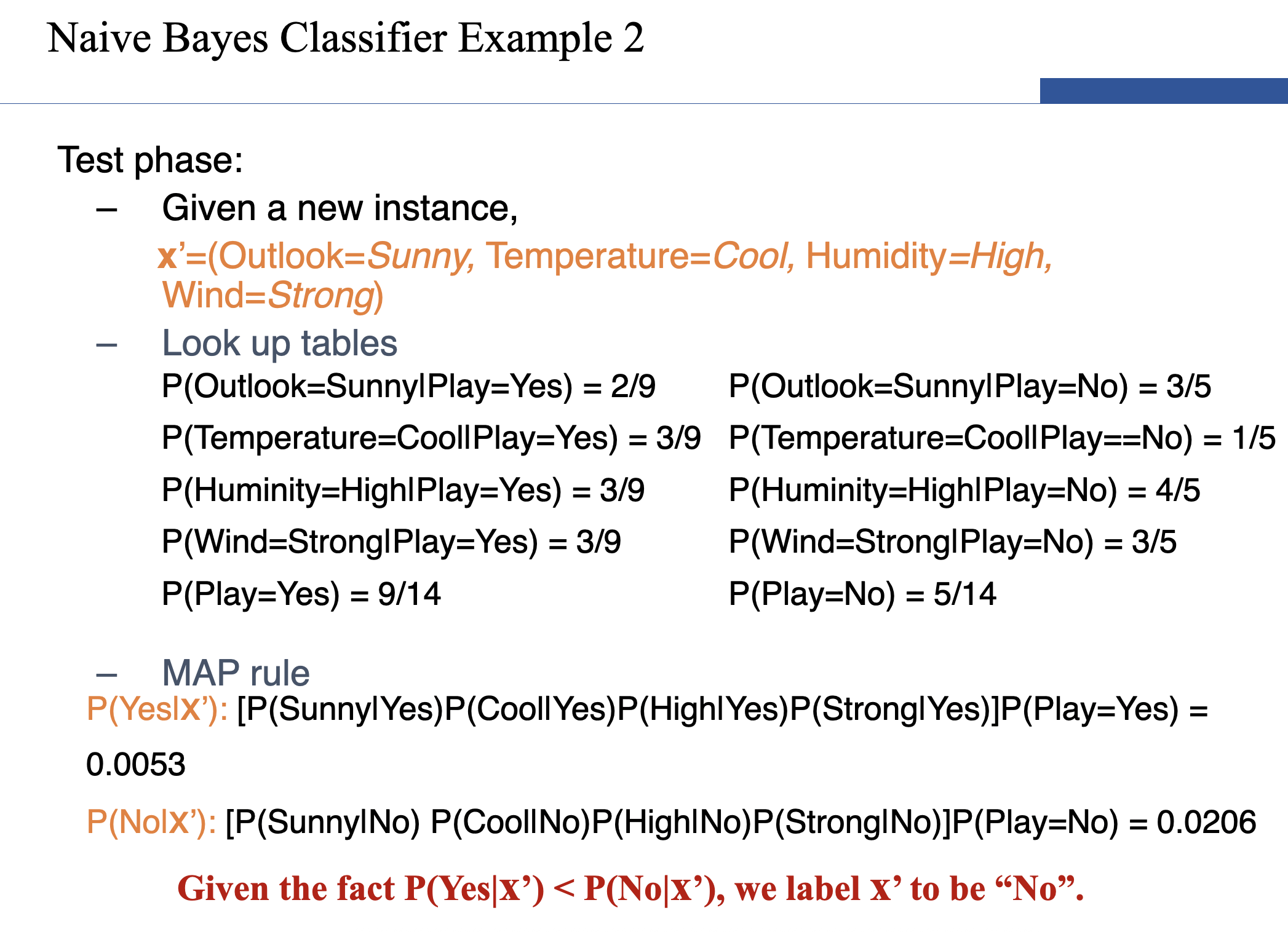
Naive Bayes

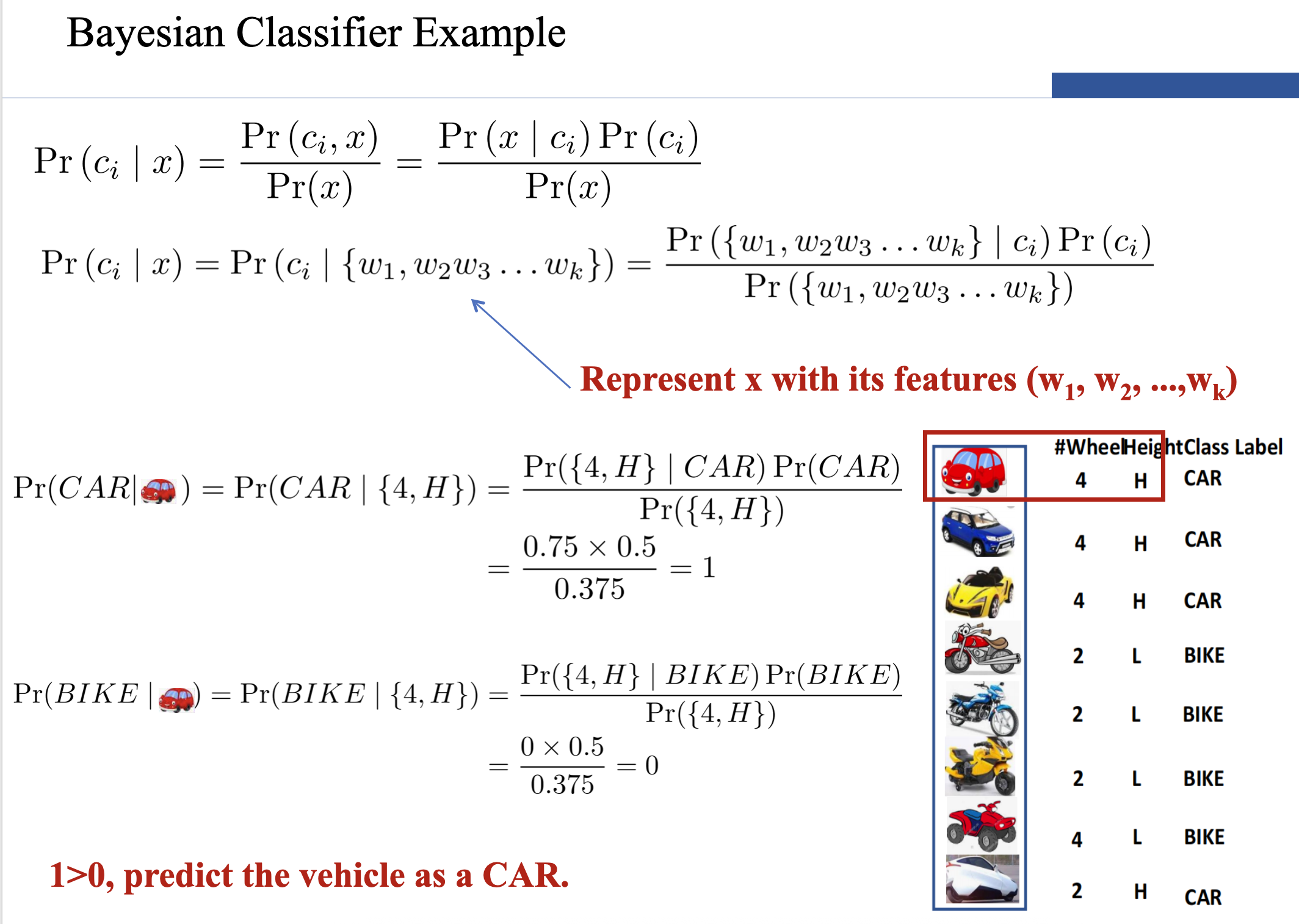
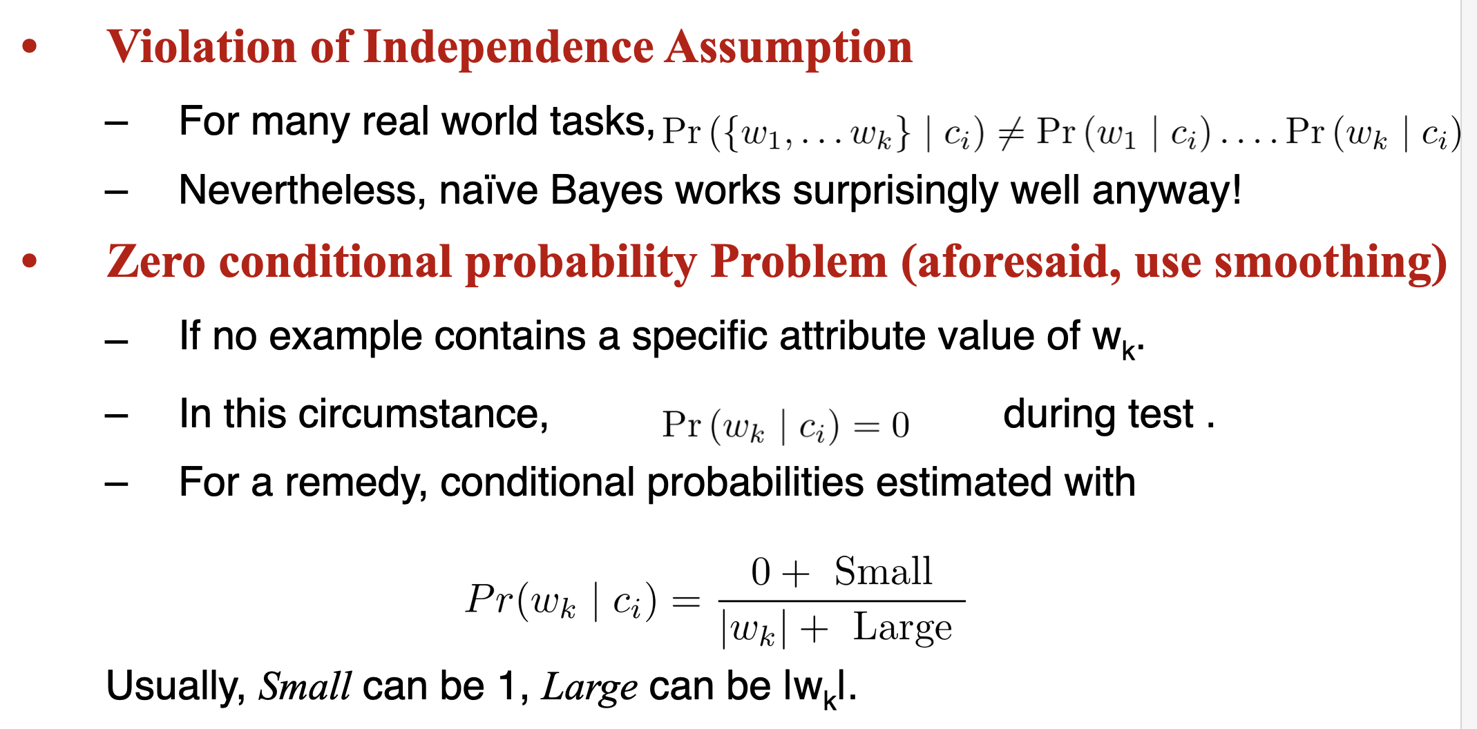
However, if k (the number of classes) is very large, estimating likelihood $Pr{(w1,w_2w_3,...,w_k)}$ is a very expensive task over a large dataset.
To simplify the estimation, we make an assumption. The features are conditionally independent.

View Repository

Kernel: Python 3 (ipykernel)

Dataset Loading

1. Loading the Dataset

In [1]:

import numpy as np
import matplotlib.pyplot as plt

In [2]:

from sklearn import datasets
iris = datasets.load_iris()

Output: Loads the Iris dataset into a Bunch object (like a dictionary).

iris.keys() lists all available components in the dataset.

In [3]:

iris.keys()

Out [3]:

dict_keys(['data', 'target', 'frame', 'target_names', 'DESCR', 'feature_names', 'filename', 'data_module'])

In [4]:

print(iris.DESCR)

Out [4]:

.. _iris_dataset:

Iris plants dataset
--------------------

**Data Set Characteristics:**

:Number of Instances: 150 (50 in each of three classes)
:Number of Attributes: 4 numeric, predictive attributes and the class
:Attribute Information:
    - sepal length in cm
    - sepal width in cm
    - petal length in cm
    - petal width in cm
    - class:
            - Iris-Setosa
            - Iris-Versicolour
            - Iris-Virginica

:Summary Statistics:

============== ==== ==== ======= ===== ====================
                Min  Max   Mean    SD   Class Correlation
============== ==== ==== ======= ===== ====================
sepal length:   4.3  7.9   5.84   0.83    0.7826
sepal width:    2.0  4.4   3.05   0.43   -0.4194
petal length:   1.0  6.9   3.76   1.76    0.9490  (high!)
petal width:    0.1  2.5   1.20   0.76    0.9565  (high!)
============== ==== ==== ======= ===== ====================

:Missing Attribute Values: None
:Class Distribution: 33.3% for each of 3 classes.
:Creator: R.A. Fisher
:Donor: Michael Marshall (MARSHALL%PLU@io.arc.nasa.gov)
:Date: July, 1988

The famous Iris database, first used by Sir R.A. Fisher. The dataset is taken
from Fisher's paper. Note that it's the same as in R, but not as in the UCI
Machine Learning Repository, which has two wrong data points.

This is perhaps the best known database to be found in the
pattern recognition literature.  Fisher's paper is a classic in the field and
is referenced frequently to this day.  (See Duda & Hart, for example.)  The
data set contains 3 classes of 50 instances each, where each class refers to a
type of iris plant.  One class is linearly separable from the other 2; the
latter are NOT linearly separable from each other.

.. dropdown:: References

  - Fisher, R.A. "The use of multiple measurements in taxonomic problems"
    Annual Eugenics, 7, Part II, 179-188 (1936); also in "Contributions to
    Mathematical Statistics" (John Wiley, NY, 1950).
  - Duda, R.O., & Hart, P.E. (1973) Pattern Classification and Scene Analysis.
    (Q327.D83) John Wiley & Sons.  ISBN 0-471-22361-1.  See page 218.
  - Dasarathy, B.V. (1980) "Nosing Around the Neighborhood: A New System
    Structure and Classification Rule for Recognition in Partially Exposed
    Environments".  IEEE Transactions on Pattern Analysis and Machine
    Intelligence, Vol. PAMI-2, No. 1, 67-71.
  - Gates, G.W. (1972) "The Reduced Nearest Neighbor Rule".  IEEE Transactions
    on Information Theory, May 1972, 431-433.
  - See also: 1988 MLC Proceedings, 54-64.  Cheeseman et al"s AUTOCLASS II
    conceptual clustering system finds 3 classes in the data.
  - Many, many more ...

In [5]:

iris.feature_names

Out [5]:

['sepal length (cm)',
 'sepal width (cm)',
 'petal length (cm)',
 'petal width (cm)']

In [6]:

iris.target_names

Out [6]:

array(['setosa', 'versicolor', 'virginica'], dtype='<U10')

In [7]:

iris.data[:5]

Out [7]:

array([[5.1, 3.5, 1.4, 0.2],
       [4.9, 3. , 1.4, 0.2],
       [4.7, 3.2, 1.3, 0.2],
       [4.6, 3.1, 1.5, 0.2],
       [5. , 3.6, 1.4, 0.2]])

In [8]:

iris.data.shape

Out [8]:

(150, 4)

In [9]:

iris.target

Out [9]:

array([0, 0, 0, 0, 0, 0, 0, 0, 0, 0, 0, 0, 0, 0, 0, 0, 0, 0, 0, 0, 0, 0,
       0, 0, 0, 0, 0, 0, 0, 0, 0, 0, 0, 0, 0, 0, 0, 0, 0, 0, 0, 0, 0, 0,
       0, 0, 0, 0, 0, 0, 1, 1, 1, 1, 1, 1, 1, 1, 1, 1, 1, 1, 1, 1, 1, 1,
       1, 1, 1, 1, 1, 1, 1, 1, 1, 1, 1, 1, 1, 1, 1, 1, 1, 1, 1, 1, 1, 1,
       1, 1, 1, 1, 1, 1, 1, 1, 1, 1, 1, 1, 2, 2, 2, 2, 2, 2, 2, 2, 2, 2,
       2, 2, 2, 2, 2, 2, 2, 2, 2, 2, 2, 2, 2, 2, 2, 2, 2, 2, 2, 2, 2, 2,
       2, 2, 2, 2, 2, 2, 2, 2, 2, 2, 2, 2, 2, 2, 2, 2, 2, 2])

In [10]:

iris.target.shape

Out [10]:

(150,)

3) Data Exploration

(1) The bellow graph shows relationship between the sepal length and width.

In [11]:

X = iris.data[:,:2] # Take out the information of the sepal length and width. 
y = iris.target
plt.scatter(X[y==0,0],X[y==0,1],color='red')
plt.scatter(X[y==1,0],X[y==1,1],color='blue')
plt.scatter(X[y==2,0],X[y==2,1],color='green')
plt.xlabel('Sepal Length (cm)')
plt.ylabel('Sepal Width (cm)')
plt.title('Sepal Length vs Sepal Width')
plt.show()

Out [11]:

(2) Now we will check relationship between the petal length and width.

In [12]:

X = iris.data[:,2:]
plt.scatter(X[y==0,0],X[y==0,1],color='red')
plt.scatter(X[y==1,0],X[y==1,1],color='blue')
plt.scatter(X[y==2,0],X[y==2,1],color='green')
plt.xlabel('Petal Length (cm)')
plt.ylabel('Petal Width (cm)')
plt.title('Petal Length vs Petal Width')
plt.show()

Out [12]:

As we can see that the Petal Features are giving a better cluster division compared to the Sepal features. This is an indication that the Petals can help in better and

accurate Predictions over the Sepal.

In [13]:

X = iris.data

In [14]:

import seaborn as sns 
correlation_matrix = np.corrcoef(iris.data, rowvar=False)

plt.figure(figsize=(8, 6)) 
sns.heatmap(correlation_matrix, 
            annot=True, 
            cmap='coolwarm', 
            linewidths=.5, 
            square=True, 
            xticklabels=iris.feature_names, 
            yticklabels=iris.feature_names)
plt.title('Iris Dataset Feature Correlation Heatmap')
plt.show()

Out [14]:

Observation

From the correlation heatmap of the Iris dataset, the following observations can be made:

Strong Positive Correlation:

Petal Length and Petal Width: The correlation coefficient is 0.96, indicating an extremely strong positive relationship. This means as petal length increases, petal width also tends to increase significantly.
Sepal Length and Petal Length/Petal Width: The correlation coefficients are 0.87 and 0.82, respectively, showing strong positive relationships. Longer sepals are associated with longer and wider petals.

Weak or No Correlation:

Sepal Width and Other Features: Sepal width shows weak or negative correlations with other features. For example:
Sepal Length: Correlation of -0.12 (very weak negative).
Petal Length/Petal Width: Correlations of -0.43 and -0.37, respectively (moderate negative relationships).

Diagonal Values:

The diagonal of the heatmap shows 1.0, which is expected as each feature is perfectly correlated with itself.

In [15]:

from sklearn.model_selection import train_test_split  # For splitting the dataset into training and testing sets

# Split the dataset into features (X) and target labels (y)
X = iris.data  # Features
y = iris.target  # Target Labels

# Define the desired test set size or the train-test split ratio
test_size = 0.3  # 30% of the dataset will be used for testing
# Alternatively, you can specify the train_test_split ratio directly:
# train_test_split_ratio = 0.7  # 70% of the dataset will be used for training

# Use train_test_split function to divide the dataset into training and testing sets
# Shuffle the data before splitting if desired (default is True)
#fixed random state for reproducibility
X_train, X_test, y_train, y_test = train_test_split(X, y, test_size=test_size, random_state=48)

# Print the sizes of the training and testing sets
print(f"Training set size: {len(X_train)} samples")
print(f"Test set size: {len(X_test)} samples")

Out [15]:

Training set size: 105 samples
Test set size: 45 samples

In [16]:

from sklearn.neighbors import KNeighborsClassifier  # K-Nearest Neighbors (KNN) classifier implementation

# Instantiate a KNN classifier with k=3 (considering 3 nearest neighbors for classification)
knn = KNeighborsClassifier(n_neighbors=3)

# Train the KNN classifier on the training data
knn.fit(X_train, y_train)

Out [16]:

KNeighborsClassifier(n_neighbors=3)

In [17]:

# Make predictions on the testing data using the trained KNN classifier
y_pred = knn.predict(X_test)
y_pred

Out [17]:

array([1, 1, 2, 0, 1, 2, 0, 1, 0, 1, 2, 0, 0, 2, 1, 1, 0, 1, 2, 2, 0, 2,
       1, 1, 2, 0, 0, 2, 2, 1, 2, 1, 2, 0, 1, 2, 2, 1, 0, 1, 1, 1, 2, 2,
       1])

In [18]:

from sklearn.metrics import accuracy_score  # For evaluating model performance

# Print the overall accuracy score (fraction of correctly classified instances)
print("\nAccuracy Score:", accuracy_score(y_test, y_pred))

Out [18]:


Accuracy Score: 0.9555555555555556

In [23]:

import pandas as pd

results = pd.DataFrame({
    'Actual': y_test,
    'Predicted': y_pred,
    'Correct': y_test == y_pred
})

# Filter to show only misclassified samples
misclassified = results[results['Correct'] == False]
print(misclassified)

Out [23]:

    Actual  Predicted  Correct
7        2          1    False
18       1          2    False

In [19]:

# Define the range of K values
k_values = np.arange(1, 11)

# Initialize a NumPy array to store the accuracy scores
accuracy_scores = np.zeros(k_values.shape)

# Iterate over K values
for i, k in enumerate(k_values):
    # Create a K-Nearest Neighbors classifier with the current K value
    knn = KNeighborsClassifier(n_neighbors=k)
    
    # Train the model on the training data
    knn.fit(X_train, y_train)
    
    # Make predictions on the test set
    predictions = knn.predict(X_test)
    
    # Compute and store the accuracy score corresponding to the current K value
    accuracy_scores[i] = accuracy_score(predictions, y_test)
    
    print("k = ", k, " Accuracy Score:", accuracy_scores[i])

# Plot the relationship between accuracy and K values using matplotlib
plt.plot(k_values, accuracy_scores)
plt.xticks(np.arange(1, 11))

Out [19]:

k =  1  Accuracy Score: 0.9555555555555556
k =  2  Accuracy Score: 0.9111111111111111
k =  3  Accuracy Score: 0.9555555555555556
k =  4  Accuracy Score: 0.9333333333333333
k =  5  Accuracy Score: 0.9555555555555556
k =  6  Accuracy Score: 0.9333333333333333
k =  7  Accuracy Score: 0.9555555555555556
k =  8  Accuracy Score: 0.9555555555555556
k =  9  Accuracy Score: 1.0
k =  10  Accuracy Score: 0.9555555555555556

([<matplotlib.axis.XTick at 0x1361eb7a0>,
  <matplotlib.axis.XTick at 0x1361b93a0>,
  <matplotlib.axis.XTick at 0x1361b8c50>,
  <matplotlib.axis.XTick at 0x1244923f0>,
  <matplotlib.axis.XTick at 0x123c369c0>,
  <matplotlib.axis.XTick at 0x1244395b0>,
  <matplotlib.axis.XTick at 0x124491dc0>,
  <matplotlib.axis.XTick at 0x12443b530>,
  <matplotlib.axis.XTick at 0x12443a7e0>,
  <matplotlib.axis.XTick at 0x12443a9c0>],
 [Text(1, 0, '1'),
  Text(2, 0, '2'),
  Text(3, 0, '3'),
  Text(4, 0, '4'),
  Text(5, 0, '5'),
  Text(6, 0, '6'),
  Text(7, 0, '7'),
  Text(8, 0, '8'),
  Text(9, 0, '9'),
  Text(10, 0, '10')])

In [20]:

X_Sepal = iris.data[:, :2]  # Take out the information of the sepal Length and width.
X_Petal = iris.data[:, 2:]  # Take out the information of the Petal Length and width.
y = iris.target  # Target Labels
test_size = 0.3  # 30% of the dataset will be used for testing
X_train_Sepal, X_test_Sepal, y_train_Sepal, y_test_Sepal = train_test_split(X_Sepal, y, test_size=test_size, random_state=0)  # sepal
X_train_Petal, X_test_Petal, y_train_Petal, y_test_Petal = train_test_split(X_Petal, y, test_size=test_size, random_state=0)  # petals

In [21]:

knn_Sepal = KNeighborsClassifier(n_neighbors=3)
knn_Sepal.fit(X_train_Sepal, y_train_Sepal)
prediction = knn_Sepal.predict(X_test_Sepal)
print('The accuracy of the KNN using Sepal is:', accuracy_score(prediction, y_test_Sepal))

knn_Petal = KNeighborsClassifier(n_neighbors=3)
knn_Petal.fit(X_train_Petal, y_train_Petal)
prediction = knn_Petal.predict(X_test_Petal)
print('The accuracy of the KNN using Petal is:', accuracy_score(prediction, y_test_Petal))

Out [21]:

The accuracy of the KNN using Sepal is: 0.7333333333333333
The accuracy of the KNN using Petal is: 0.9777777777777777