Lesson 1.4: Neural Networks

Neural networks are machine learning models that mimic the complex functions of the human brain. These models consist of interconnected nodes or neurons that process data, learn patterns, and enable tasks such as pattern recognition and decision-making.

Neural networks are capable of learning and identifying patterns directly from data without pre-defined rules. These networks are built from several key components:

Neurons: The basic units that receive inputs, each neuron is governed by a threshold and an activation function.
Connections: Links between neurons that carry information, regulated by weights and biases.
Weights and Biases: These parameters determine the strength and influence of connections.
Propagation Functions: Mechanisms that help process and transfer data across layers of neurons.
Learning Rule: The method that adjusts weights and biases over time to improve accuracy.

Learning in neural networks follows a structured, three-stage process:

Input Computation: Data is fed into the network.
Output Generation: Based on the current parameters, the network generates an output.
Iterative Refinement: The network refines its output by adjusting weights and biases, gradually improving its performance on diverse tasks.

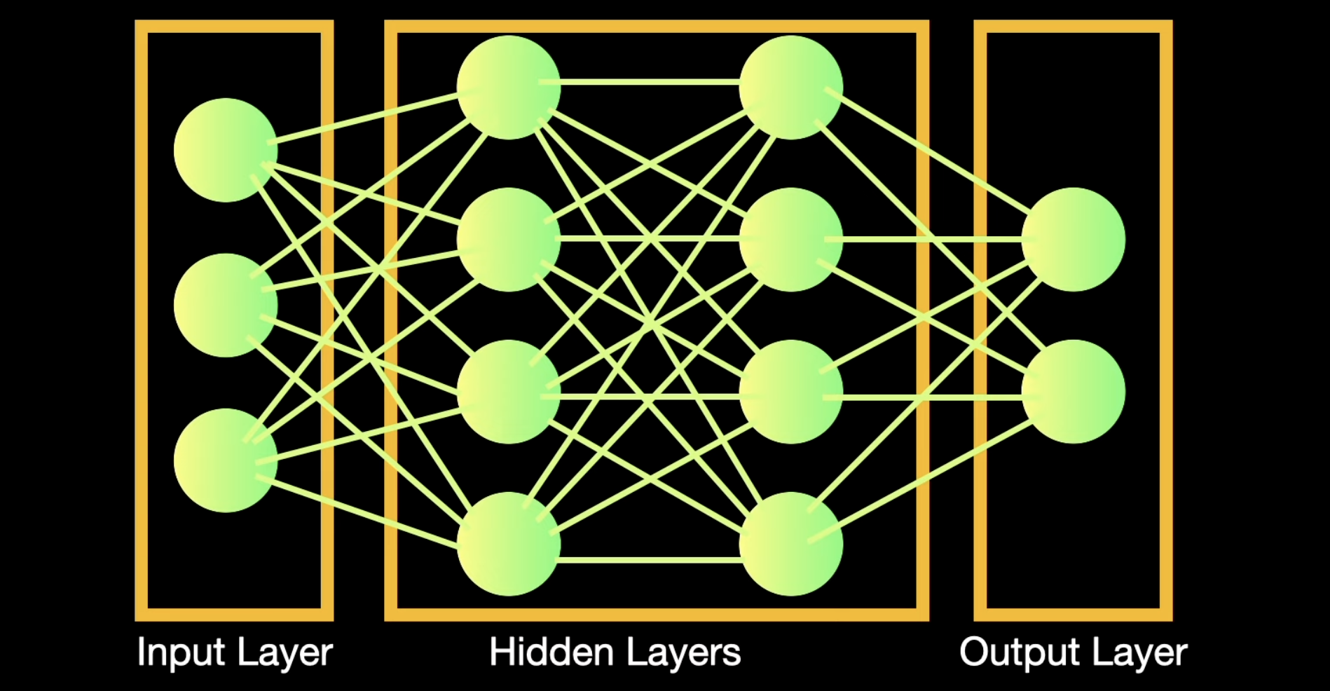
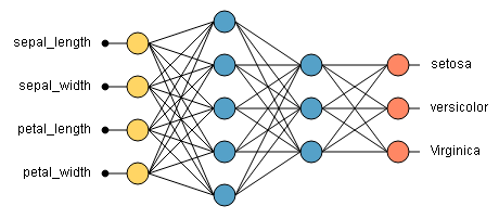
Layers in Neural Network Architecture

Input Layer:

This is where the network receives its input data. Each input neuron in the layer corresponds to a feature in the input data.
- The input layer consists of neurons (or nodes), each representing a feature of the input data.
- For example, if the input is an image with 784 pixels (e.g., a 28x28 grayscale image), the input layer will have 784 neurons, each representing one pixel value.
- The input layer does not perform any computation; it simply passes the data to the first hidden layer.

Hidden Layers:

These layers perform most of the computational heavy lifting. A neural network can have one or multiple hidden layers. Each layer consists of units (neurons) that transform the inputs into something that the output layer can use.
- Each hidden layer consists of neurons that perform two key operations:
  1. Weighted Sum: Compute the weighted sum of inputs from the previous layer
  2. Activation Function: Apply a non-linear activation function (e.g., ReLU, sigmoid, tanh) to introduce non-linearity
- The output of each neuron in the hidden layer is passed to the next layer.
- Multiple hidden layers allow the network to learn hierarchical features:
  - Early layers learn simple patterns (e.g., edges in an image).
  - Deeper layers learn complex patterns (e.g., shapes, objects).

Output Layer:

The final layer produces the output of the model. The format of these outputs varies depending on the specific task (e.g., classification, regression). The output layer consists of neurons that represent the final output of the network.
- The number of neurons in the output layer depends on the task:
  - Binary Classification: 1 neuron (outputs a probability between 0 and 1).
  - Multi-Class Classification: $n$ neurons (one for each class, outputs probabilities for each class).
  - Regression: 1 neuron (outputs a continuous value).
- The output layer computes the weighted sum of inputs from the last hidden layer and applies an appropriate activation function:
  - Sigmoid: For binary classification (outputs a probability between 0 and 1).
  - Softmax: For multi-class classification (outputs probabilities for each class).
  - Linear/Identity: For regression (outputs a continuous value).

Working of Neural Networks

Forward Propagation

When data is input into the network, it passes through the network in the forward direction, from the input layer through the hidden layers to the output layer. This process is known as forward propagation. Here’s what happens during this phase:

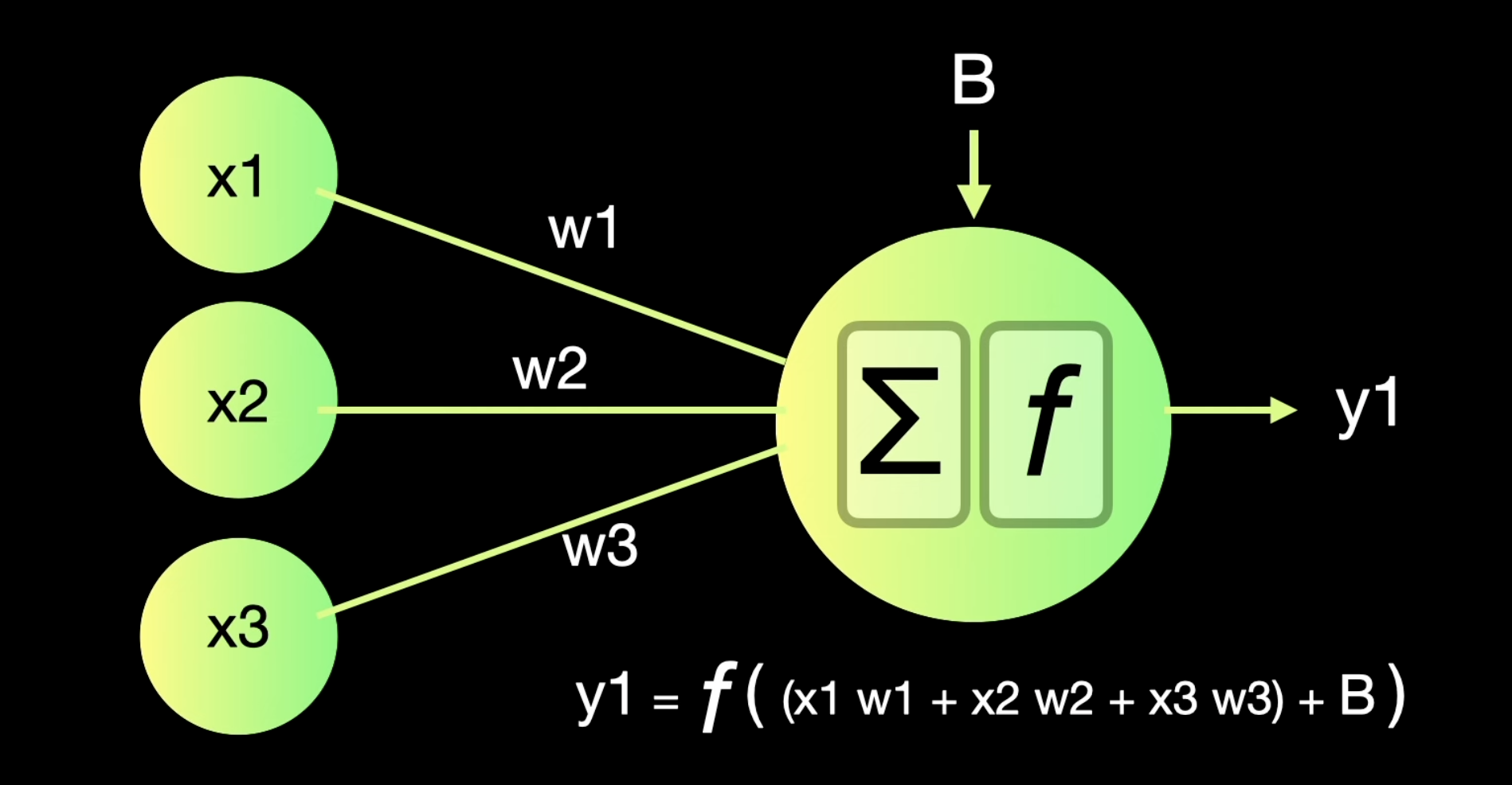
Linear Transformation: Each neuron in a layer receives inputs, which are multiplied by the weights associated with the connections. These products are summed together, and a bias is added to the sum. This can be represented mathematically as:

$z = w_1x_1 + w_2x_2 + \dots + w_nx_n + b$ where
$w$ represents the weights,
$x$ represents the inputs, and
$b$ is the bias is then passed through an activation function. The activation function is crucial because it introduces non-linearity into the system, enabling the network to learn more complex patterns. Popular activation functions include ReLU, sigmoid, and tanh.

Activation: The result of the linear transformation (denoted as $z$ ) is then passed through an activation function. The activation function is crucial because it introduces non-linearity into the system, enabling the network to learn more complex patterns. Popular activation functions include ReLU, sigmoid, and tanh.

Backpropagation

After forward propagation, the network evaluates its performance using a loss function, which measures the difference between the actual output and the predicted output. The goal of training is to minimize this loss. This is where backpropagation comes into play:

Loss Calculation: The network calculates the loss, which provides a measure of error in the predictions. The loss function could vary; common choices are mean squared error for regression tasks or cross-entropy loss for classification.
Gradient Calculation: The network computes the gradients of the loss function with respect to each weight and bias in the network. This involves applying the chain rule of calculus to find out how much each part of the output error can be attributed to each weight and bias.
Weight Update: Once the gradients are calculated, the weights and biases are updated using an optimization algorithm like stochastic gradient descent (SGD). The weights are adjusted in the opposite direction of the gradient to minimize the loss. The size of the step taken in each update is determined by the learning rate.

Iteration

This process of forward propagation, loss calculation, backpropagation, and weight update is repeated for many iterations over the dataset. Over time, this iterative process reduces the loss, and the network’s predictions become more accurate.

Through these steps, neural networks can adapt their parameters to better approximate the relationships in the data, thereby improving their performance on tasks such as classification, regression, or any other predictive modeling.

Example Problem: Predicting the effectiveness of a drug dosage.

Dosages: Low (0), Medium (1), High (0).
Goal: Predict whether a future dosage will be effective.
Challenge: A straight line cannot accurately predict all three dosages.
Solution: A neural network can fit a "squiggle" (non-linear function) to the data, allowing it to model complex relationships.

let's imagine we tested a drug that was designed to treat an illness and we gave the drug to three different groups of people, with three different dosages: low, medium, and high.

The low dosages were not effective so we set them to 0 on this graph.
The medium dosages were effective so we set them to 1.
The high dosages were not effective, so those are set to 0. now that we have this data, we would like to use it to predict whether or not a future dosage will be effective.

Structure of a Neural Network

Nodes and Connections:
- A neural network consists of nodes (neurons) and connections (synapses) between them.
- Each connection has a weight (parameter) that is estimated during training.
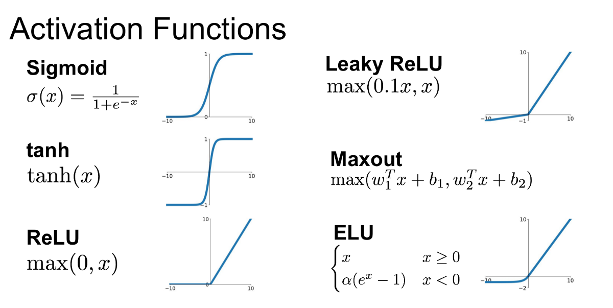
Activation Functions:
- Nodes in the hidden layers use activation functions to introduce non-linearity.
- Common activation functions:
  - Softplus: $f(x) = log(1 + e^x)$
  - ReLU (Rectified Linear Unit): $f(x) = max(0,x)$
  - Sigmoid: $f(x) = \frac{1}{1+e^-x}$

Neural Network Components

Input Layer:
- Contains the input features (e.g., drug dosage).
Hidden Layers:
- Layers between the input and output layers.
- Each node in the hidden layer applies an activation function to a weighted sum of its inputs.
Output Layer:
- Produces the final prediction (e.g., drug effectiveness).

It only has one input node, where we plug in the dosage, only one output node to tell us the predicted effectiveness, and only two nodes between the input and output nodes. These layers of nodes between the input and output nodes are called hidden layers. When you build a neural network one of the first things you do is decide how many hidden layers you want and how many nodes go into each hidden layer. Although there are rules of thumb for making decisions about the hidden layers, you essentially make a guess and see how well the neural network performs, adding more layers and nodes if needed. Now, even though this neural network looks fancy, it is still made from the same parts used in this simple neural network, which has only one hidden layer with two nodes.

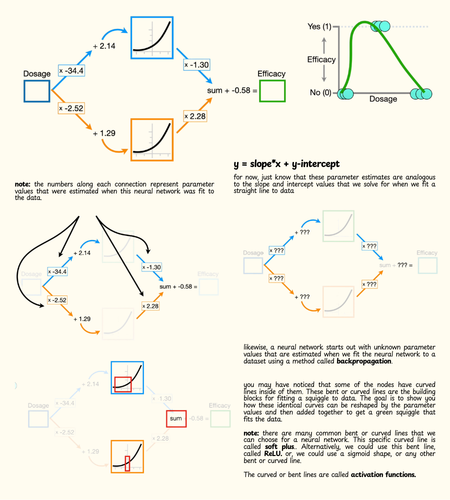
A neural network starts out with unknown parameter values that are estimated when we fit the neural network to a dataset using a method called backpropagation. but, for now, just assume that we've already fit this neural network to this specific dataset, and that means we have already estimated these parameters.
Also, you may have noticed that some of the nodes have curved lines inside of them, these bent or curved lines are the building blocks for fitting a squiggle to data.
The goal of this example is to show you how these identical curves can be reshaped by the parameter values and then added together to get a green squiggle that fits the data.
Note: There are many common bent or curved lines that we can choose for a neural network. This specific curved line is called soft plus. Alternatively, we could use this bent line, called ReLU or, we could use a sigmoid shape, or any other bent or curved line. Thes curved or bent lines are called activation functions.

BLUE CURVE

Note: To keep the math simple, let's assume dosages go from zero, for low, to one, for high.
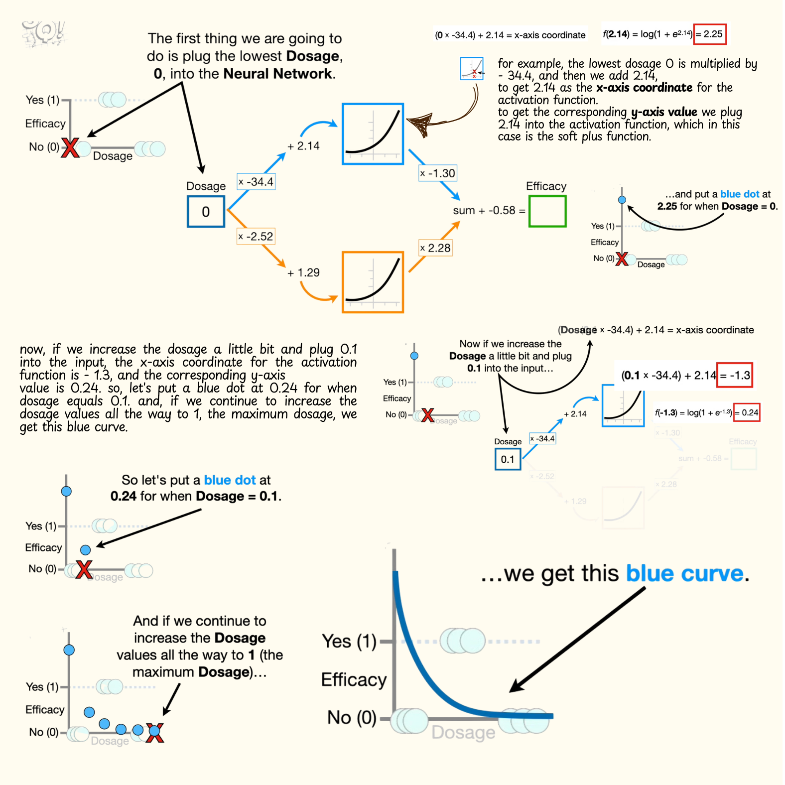
The first thing we are going to do is plug the lowest dosage, zero, into the neural network.
To get from the input node to the top node in the hidden layer, this connection multiplies the dosage by negative 34.4 and then adds 2.14, and the result is an x-axis coordinate for the activation function.
- The lowest dosage 0 is multiplied by negative 34.4, and then we add 2.14, to get 2.14 as the x-axis coordinate for the activation function.
- To get the corresponding y-axis value we plug 2.14 into the activation function, which in this case is the soft plus function. Note: if we had chosen the sigmoid curve for the activation function then we would plug 2.14 into the equation for the sigmoid curve, and if we had chosen the ReLU bent line for the activation function, then we would plug 2.14 into the ReLU equation.
- The log of one plus e raised to the 2.14 power is 2.25.
note: in statistics, machine learning, and most programming languages, the log function implies the natural log, or the log base e. anyway, the y-axis coordinate for the activation function is 2.25, so let's extend this y-axis up a little bit and put a blue dot at 2.25 for when dosage equals zero.
Now, if we increase the dosage a little bit and plug 0.1 into the input, the x-axis coordinate for the activation function is negative 1.3, and the corresponding y-axis value is 0.24. so, let's put a blue dot at 0.24 for when dosage equals 0.1.
- if we continue to increase the dosage values all the way to 1, the maximum dosage, we get this blue curve.
Note: before we move on I want to point out that the full range of dosage values, from 0 to 1, corresponds to this relatively narrow range of values from the activation function. in other words, when we plug dosage values, from 0 to 1, into the neural network, and then multiply them by negative 34.4 and add 2.14, we only get x-axis coordinates that are within the red box. and thus, only the corresponding y-axis values in the red box are used to make this new blue curve.
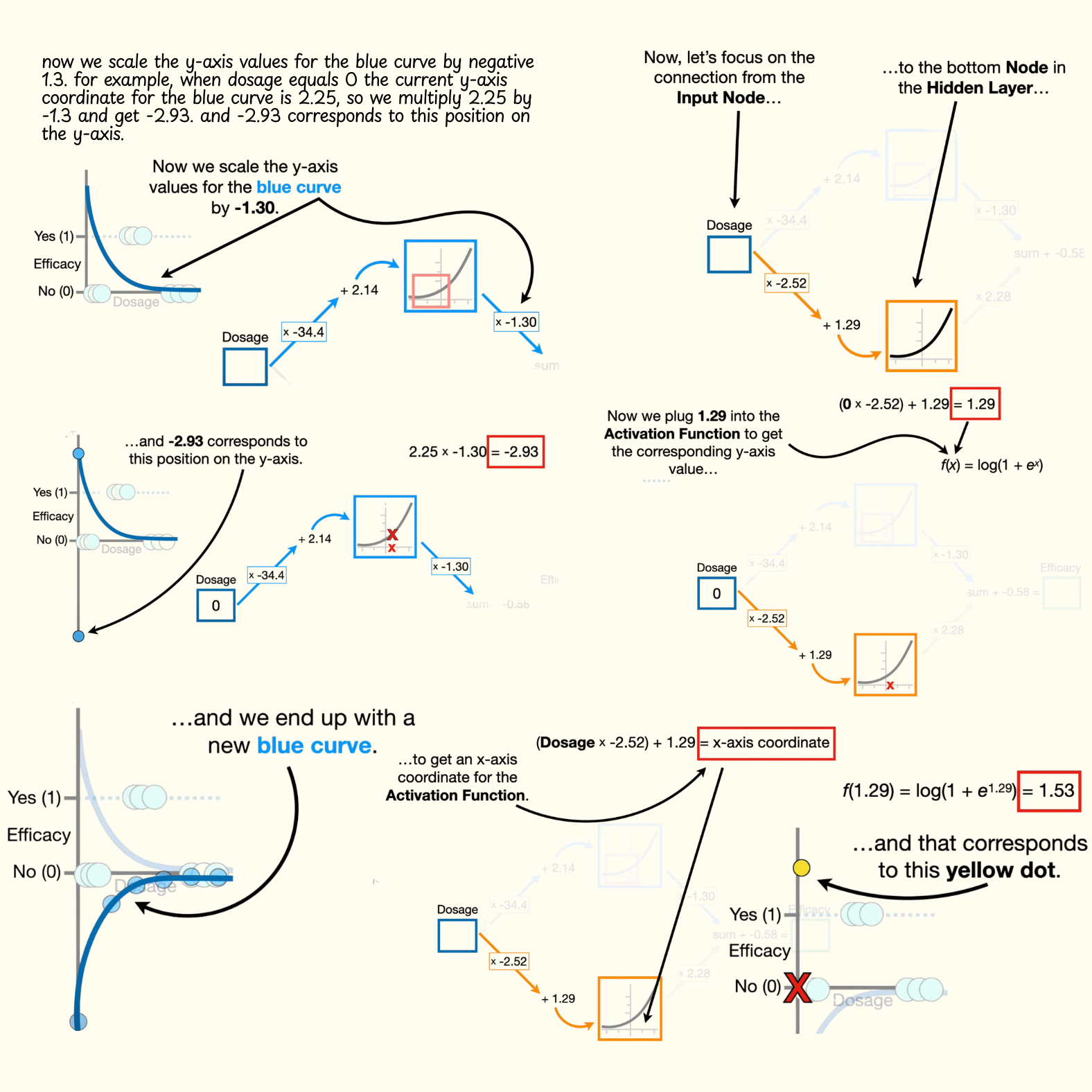
Now we scale the y-axis values for the blue curve by negative 1.3. for example, when dosage equals zero the current y-axis coordinate for the blue curve is 2.25, so we multiply 2.25 by negative 1.3 and get negative 2.93. and negative 2.93 corresponds to this position on the y-axis. likewise, we multiply all of the other y-axis coordinates on the blue curve by negative 1.3 and we end up with a new blue curve.

YELLOW CURVE

Now, let's focus on the connection from the input node, to the bottom node in the hidden layer. however, this time, we multiply the dosage by negative 2.52, instead of negative 34.4, and we add 1.29, instead of 2.14, to get the x-axis coordinate for the activation function. remember, these values come from fitting the neural network to the data with backpropagation, and we'll talk about that in part two in this series.
Now, if we plug the lowest dosage, zero, into the neural network, then the x-axis coordinate for the activation function is 1.29.
Now we plug 1.29 into the activation function to get the corresponding y-axis value, and get 1.53. and that corresponds to this yellow dot.
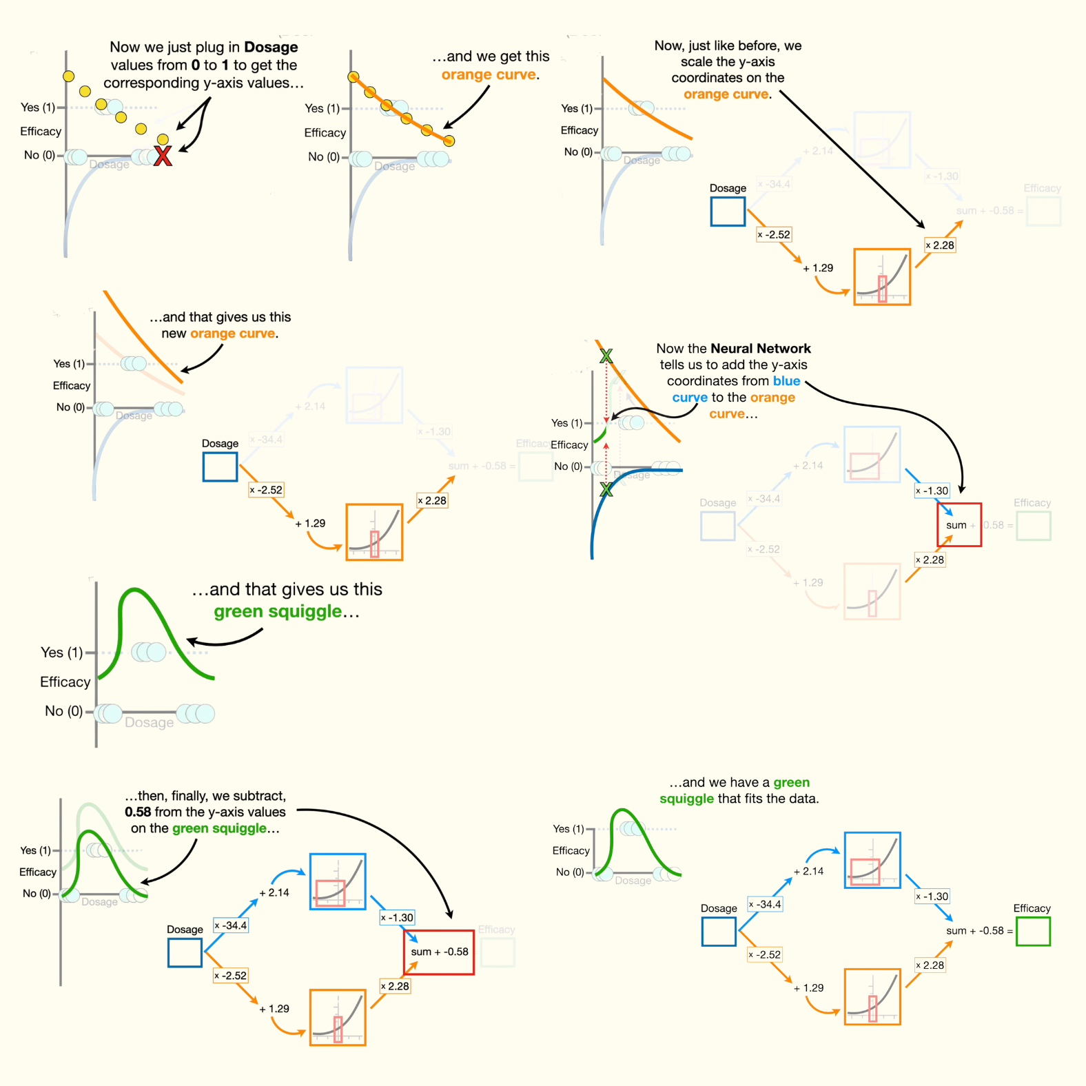
Now, we just plug in dosage values from 0 to 1 to get the corresponding y-axis values, and we get this orange curve.
Note: Just like before, i want to point out that the full range of dosage values, from 0 to 1, corresponds to this narrow range of values from the activation function. in other words, when we plug dosage values from 0 to 1 into the neural network we only get x-axis coordinates that are within the red box and thus, only the corresponding y-axis values in the red box are used to make this new orange curve.
So we see that fitting a neural network to data gives us different parameter estimates on the connections and that results in each node in the hidden layer using different portions of the activation functions to create these new and exciting shapes. now, just like before, we scale the y-axis coordinates on the orange curve, only this time we scale by a positive number: 2.28.

GREEN SQUIGGLE

Now the neural network tells us to add the y-axis coordinates from the blue curve to the orange curve, and that gives us this green squiggle.
Then, finally, we subtract 0.58 from the y-axis values on the green squiggle, and we have a green squiggle that fits the data.
Now, if someone comes along and says that they are using dosage equal to 0.5 we can look at the corresponding y-axis coordinate on the green squiggle and see that the dosage will be effective. or, we can solve for the y-axis coordinate by plugging dosage equals 0.5 into the neural network, and do the math.

Now, if you've made it this far you may be wondering why this is called a neural network. instead of a big fancy squiggle fitting machine. the reason is that way back in the 1940s and 50s, when neural networks were invented, they thought the nodes were vaguely like neurons, and the connections between the nodes were sort of like synapses however, i think they should be called big fancy squiggle fitting machines, because that's what they do.

Note: whether or not you call it a squiggle fitting machine, the parameters that we multiply are called weights, and the parameters that we add are called biases.
Note: this neural network starts with two identical activation functions, but the weights and biases on the connections slice them, flip them, and stretch them into new shapes, which are then added together to get a squiggle that is entirely new and then the squiggle is shifted to fit the data.
Now, if we can create this green squiggle with just two nodes in a single hidden layer, just imagine what types of green squiggles we could fit with more hidden layers and more nodes in each hidden layer. in theory, neural networks can fit a green squiggle to just about any dataset, no matter how complicated, and i think that's pretty cool.

Backpropagation

So let's talk about how backpropagation optimizes the weights and biases in this, and other, neural networks. In this part we talk about the main ideas of backpropagation.

Using the chain rule to calculate derivatives
- $\frac{\text{d SSR}}{\text{d bias}} = \frac{\text{d SSR}}{\text{d Predicted}} * \frac{\text{d Predicted}}{\text{d bias}}$
Plugging the derivatives

First, so we can be clear about which specific weights we are talking about, let's give each one a name: we have w1, w2, w3, and w4 and let's name each bias: b1, b2, and b3.

Note: conceptually, backpropagation starts with the last parameter and works its way backwards to estimate all of the other parameters. However, we can discuss all of the main ideas behind a backpropagation by just estimating the last bias, b3. So, in order to start from the back, let's assume that we already have optimal values for all of the parameters except for the last bias term, b3.
Note: throughout this, I'll make the parameter values that have already been optimized green, and unoptimized parameters will be red.
Note: To keep the math simple, let's assume dosages go from 0, for low, to 1, for high.

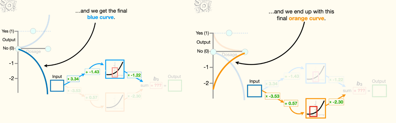
Then we multiply the y-axis coordinates on the blue curve by negative 1.22 and we get the final blue curve. Now, if we run dosages from zero to one through the connection to the bottom node in the hidden layer, then we get x-axis coordinates inside this red box. Now we plug those x-axis coordinates into the activation function to get the corresponding y-axis coordinates for this orange curve. Now we multiply the y-axis coordinates on the orange curve by negative 2.3 and we end up with this final orange curve.

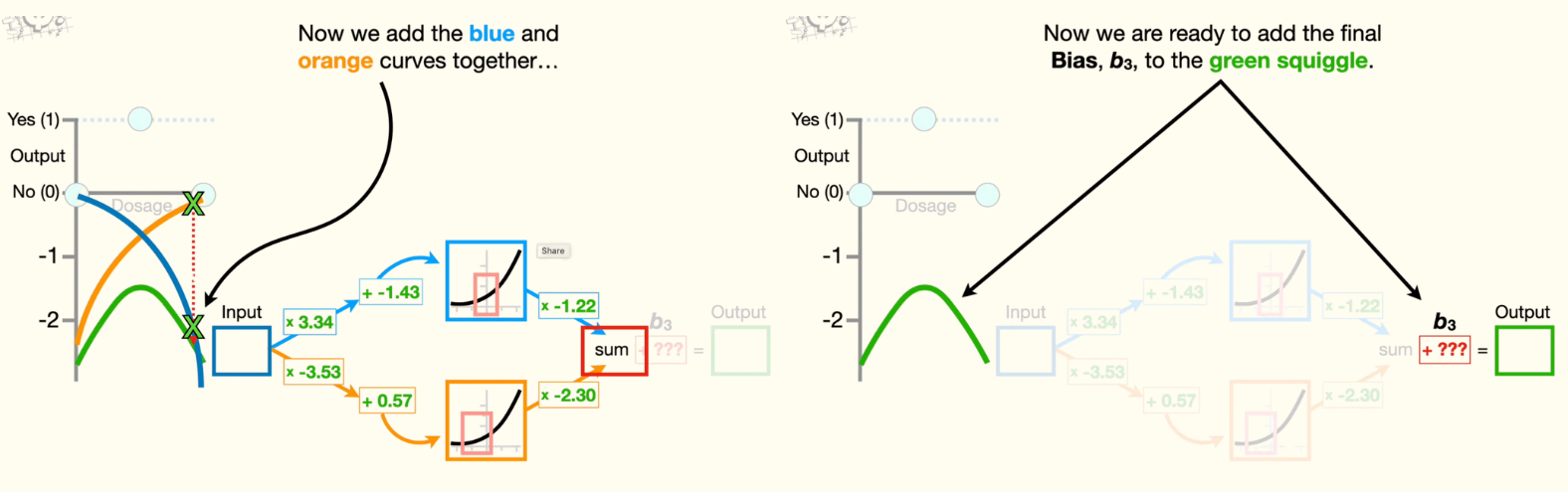
Now we add the blue and orange curves together to get this green squiggle. Now we are ready to add the final bias, b3, to the green squiggle. Because we don't yet know the optimal value for b3, we have to give it an initial value, and because bias terms are frequently initialized to 0, we will set b3 equal to 0. Now, adding zero to all of the y-axis coordinates on the green squiggle leaves it right where it is. However, that means the green squiggle is pretty far from the data that we observed.

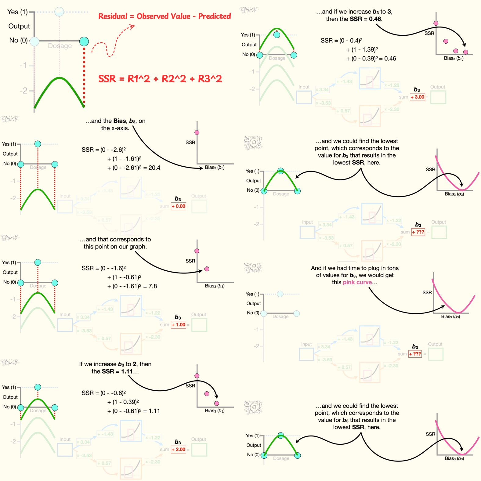
We can quantify how good the green squiggle fits the data by calculating the sum of the squared residuals. A residual is the difference between the observed and predicted values.

First residual is the observed value, zero, minus the predicted value from the green squiggle, negative 2.6.
Second residual is the observed value, one, minus the predicted value from the green squiggle, negative 1.61.
Lastly, Third this residual is the observed value, 0, minus the predicted value from the green squiggle, negative 2.61.
Now we square each residual and add them all together to get 20.4 for the sum of the squared residuals. So when b3 equals 0, the sum of the squared residuals equals 20.4. And that corresponds to this location on this graph that has the sum of the squared residuals on the y -axis and the bias, b3, on the x-axis.
Now, if we increase b3 to 1, then we would add one to the y-axis coordinates on the green squiggle and shift the green squiggle up one. And we end up with shorter residuals. When we do the math, the sum of the squared residuals equals 7.8, and that corresponds to this point on our graph.
If we increase b3 to 2, then the sum of the squared residuals equals 1.11. And if we increase b3 to 3, then the sum of the squared residuals equals 0.46.
And if we had time to plug in tons of values for b3, we would get this pink curve, and we could find the lowest point, which corresponds to the value for b3 that results in the lowest sum of the squared residuals, here. However, instead of plugging in tons of values to find the lowest point in the pink curve, we use gradient descent to find it relatively quickly.

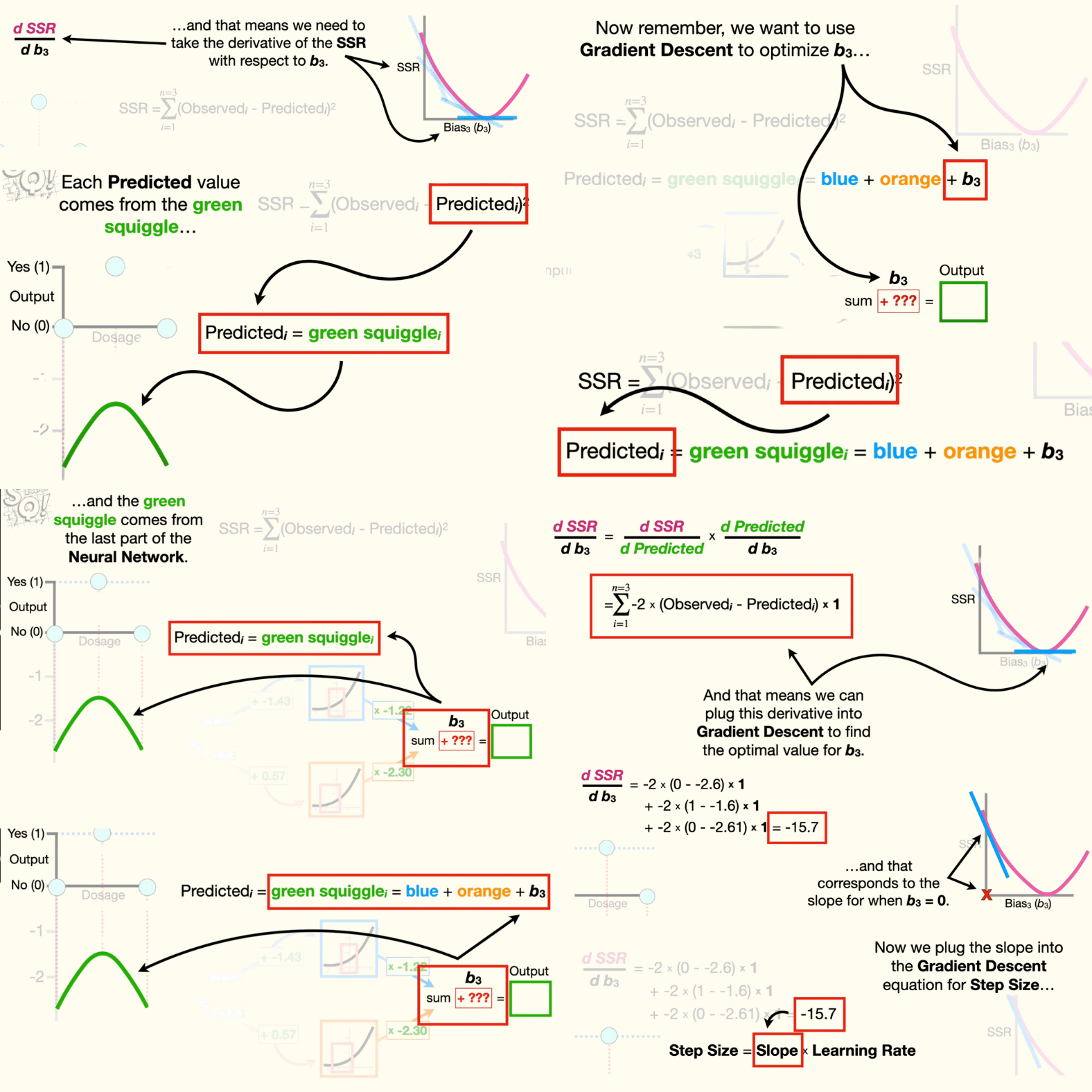
And that means we need to find the derivative of the sum of the squared residuals with respect to b3. Now, remember the sum of the squared residuals equals the first residual squared, plus all of the other squared residuals.
Now, because this equation takes up a lot of space, we can make it smaller by using summation notation. The greek symbol sigma tells us to sum things together, and 'i' is an index for the observed and predicted values that starts at one. And the index goes from one to the number of values, 'n', which in this case is set to 3. So, when 'i' equals one, we're talking about the first residual. When 'i' equals two, we're talking about the second residual And when 'i' equals three, we are talking about the third residual.
Now let's talk a little bit more about the predicted values. Each predicted value comes from the green squiggle, and the green squiggle comes from the last part of the neural network. In other words, the green squiggle is the sum of the blue and orange curves, plus b3.
Now remember, we want to use gradient descent to optimize b3, and that means we need to take the derivative of the sum of the squared residuals with respect to b3. And because the sum of the squared residuals are linked to b3 by the predicted values, we can use the chain rule to solve for the derivative of the sum of the squared residuals with respect to b3. The chain rule says that the derivative of the sum of the squared residuals with respect to b3 is the derivative of the sum of the squared residuals with respect to the predicted values, times the derivative of the predicted values with respect to b3.
Now we can solve for the derivative of the sum of the squared residuals with respect to the predicted values by first substituting in the equation, and then use the chain rule to move the square to the front, and then we multiply that by the derivative of the stuff inside the parentheses with respect to the predicted values, negative one.
Now we simplify by multiplying two by negative 1, and we have the derivative of the sum of the squared residuals with respect to the predicted values.
Now let's solve for the second part: the derivative of the predicted values with respect to b3. We start by plugging in the equation for the predicted values. Remember, the blue and orange curves were created before we got to b3. So the derivative of the blue curve with respect to b3 is 0, because the blue curve is independent of b3. And the derivative of the orange curve with respect to b3 is also 0. Lastly, the derivative of b3, with respect to b3, is 1.
Now we just add everything up, and the derivative of the predicted values with respect to b3, is one. So we multiply the derivative of the sum of the squared residuals with respect to the predicted values by 1.
- Note: this times 1 part in the equation doesn't do anything, but I'm leaving it in to remind us that the derivative of the sum of the squared residuals with respect to b3 consists of two parts: the derivative of the sum of the squared residuals with respect to the predicted values, and the derivative of the predicted values with respect to b3. And at long last we have the derivative of the sum of the squared residuals with respect to b3.
And that means we can plug this derivative into gradient descent to find the optimal value for b3. So let's move this equation up and show how we can use this equation with gradient descent.
Anyway, first, we expand the summation. Then, we plug in the observed values and the values predicted by the green squiggle. Remember, we get the predicted values on the green squiggle by running the dosages through the neural network. Now, we just do the math and get negative 15.7. And that corresponds to the slope for when b3 equals zero.

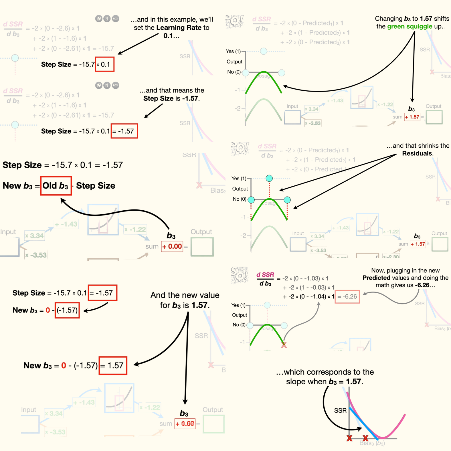
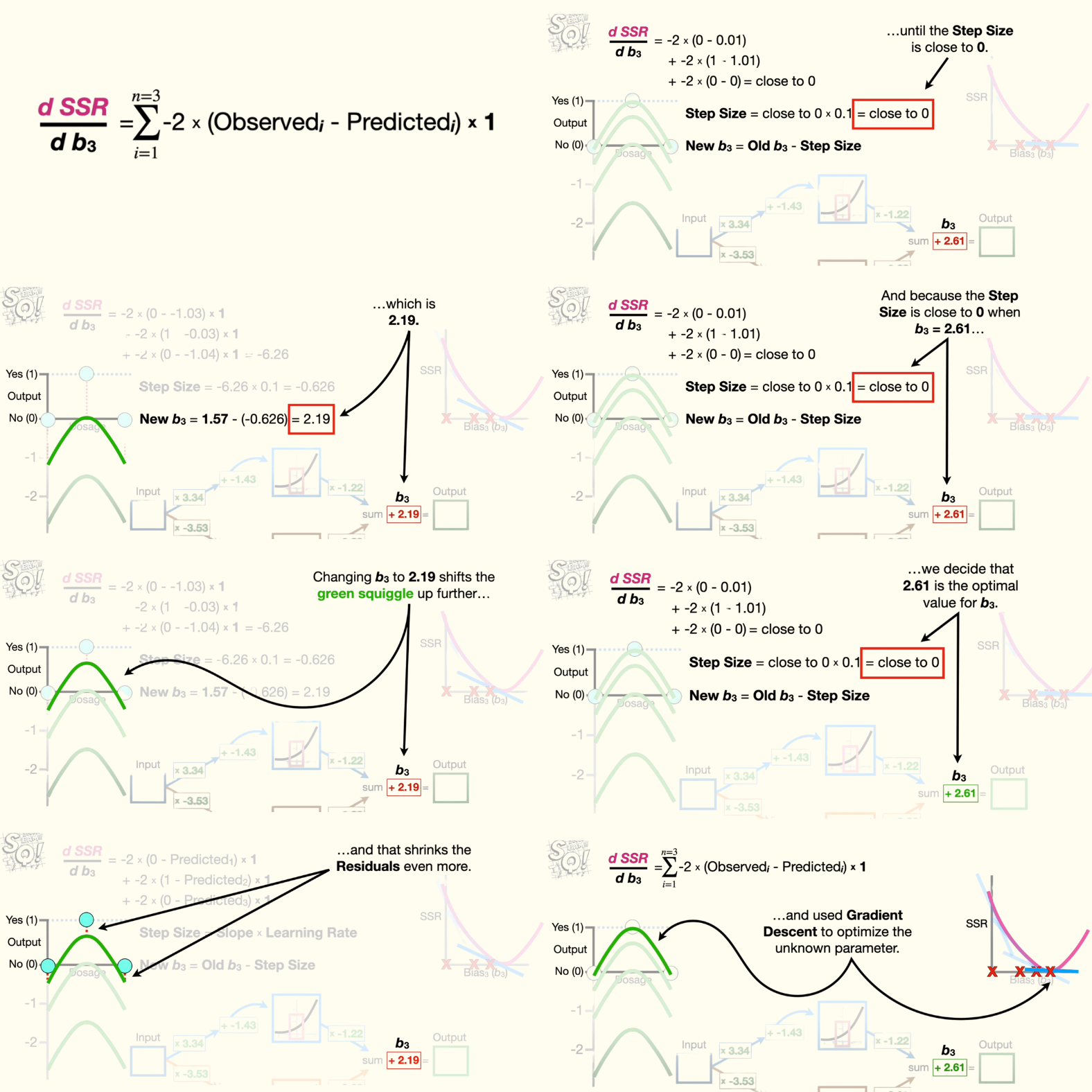
Now we plug the slope into the gradient descent equation for step size, and, in this example, we'll set the learning rate to 0.1. And that means the step size is -1.57.
Now we use the step size to calculate the new value for b3 by plugging in the current value for b3, zero, and the step size, -1.57. And the new value for b3 is 1.57. Changing b3 to 1.57 shifts the green squiggle up, and that shrinks the residuals.
Now, plugging in the new predicted values and doing the math gives us -6.26, which corresponds to the slope when b3 equals 1.57. Then, we calculate the step size and the new value for b3, which is 2.19. Changing b3 to 2.19 shifts the green squiggle up further, and that shrinks the residuals even more.
Now we just keep taking steps until the step size is close to zero. And because the step size is close to 0 when b3 equals 2.61, we decide that 2.61 is the optimal value for b3.

So, the main ideas for backpropagation are that, when a parameter is unknown, like b3, we use the chain rule to calculate the derivative of the sum of the squared residuals with respect to the unknown parameter, which in this case was b3. Then we initialize the unknown parameter with a number, and in this case we set b3 equal to zero, and used gradient descent to optimize the unknown parameter.

Optimizing All Parameters in Neural Networks

In a neural network, all weights and biases are optimized simultaneously during backpropagation, even though they might seem interconnected. Think of it like tuning a complex machine with many dials (parameters). When you adjust one dial (like a bias term), it affects how the other dials (weights and biases in earlier layers) need to be tuned to improve performance. Instead of fixing one parameter at a time, the network uses the chain rule to trace how every parameter contributes to the final error, starting from the output and working backward. Each weight and bias in hidden layers gets updated based on its role in propagating errors forward. Even after calculating an optimal value for a bias, the process continues iteratively—adjusting all parameters in small steps, over many cycles, until the network’s predictions align with the data. This ensures the entire system learns holistically, balancing all parts together rather than in isolation

References:

View Repository

Kernel: .venv

Iris Flower Classification Neural Network with PyTorch

A lightweight 3-layer neural network implemented in PyTorch for classifying Iris flower species (setosa, versicolor, virginica) based on four morphological features (sepal length/width, petal length/width). The model demonstrates:

Architecture: Input layer (4 nodes) → Hidden Layer 1 (8 nodes, ReLU) → Hidden Layer 2 (9 nodes, ReLU) → Output Layer (3 nodes)
Training: Uses Adam optimizer (lr=0.01) with CrossEntropyLoss over 100 epochs
Performance: Achieves ~95%+ accuracy with proper initialization (random_state=32)

In [41]:

import torch 
import torch.nn as nn
import torch.nn.functional as F

in features: sepal length, sepal width, petal length, petal width
out features: Iris Setosa, Iris Versicolour, or Iris Virginica

In [42]:

class Model(nn.Module):
    # Input Layer (4 features of flowers) --> HL1 (number of neurons) --> HL2(n) --> Ouput(3 Classes of Iris Flower)
    # fc -- fully connected 1 , fully connected 2 
    def __init__(self, in_features=4, h1=8, h2=9, out_features=3):
        super().__init__()
        self.fc1 = nn.Linear(in_features,h1)    # start from in_features and move to h1 , fc(fully connected)
        self.fc2 = nn.Linear(h1,h2)             # start from h1 and move to h2 
        self.out = nn.Linear(h2,out_features)   # start from h2 and move to out_features 
        
                                                # Relu stands for rectified linear unit
    def forward(self,x):
        x = F.relu(self.fc1(x))                 # if output is less than 0 , then use 0 , else leave what it is. 
        x = F.relu(self.fc2(x))                 # if output is less than 0 , then use 0 , else leave what it is. 
        x = self.out(x)
        return x

forward function in your code implements forward propagation in the neural network. Here's a breakdown of how it works:

Takes Input x:

x represents the input data (e.g., 4 features of Iris flowers: sepal length, width, petal length, width).

Passes Through Layers:

Step 1:

x = F.relu(self.fc1(x))
Input x is passed through the first fully connected layer (fc1), then the ReLU activation function is applied.
ReLU replaces negative values with 0 and keeps positive values unchanged.

Step 2:

x = F.relu(self.fc2(x))
The output from fc1 is passed through the second fully connected layer (fc2), followed by another ReLU.

Step 3: x = self.out(x)

The final layer (out) produces raw scores (logits) for the 3 Iris flower classes without activation (no softmax here!).

Returns Output:

The raw scores (logits) for each class are returned. These will later be fed into a loss function (e.g., CrossEntropyLoss, which internally applies softmax).

Here's a complete example with actual numbers to show how the calculations work in your Iris classifier:

Example Input (1 Iris flower with 4 features):

x = [5.1, 3.5, 1.4, 0.2]  # sepal_len, sepal_wid, petal_len, petal_wid

Layer 1 (fc1) Parameters:

Let's assume these random weights and biases were initialized:

Weights (8×4 matrix):

``W1 = [ [0.1, -0.2, 0.3, -0.4], # Neuron 1 weights [0.5, -0.1, 0.2, -0.3], # Neuron 2 weights [-0.2, 0.3, -0.1, 0.4], # Neuron 3 weights [0.4, -0.3, 0.2, -0.1], # Neuron 4 weights [0.2, 0.1, -0.3, 0.4], # Neuron 5 weights [-0.1, 0.4, -0.2, 0.3], # Neuron 6 weights [0.3, -0.4, 0.1, -0.2], # Neuron 7 weights [-0.3, 0.2, -0.4, 0.1] # Neuron 8 weights ]

**Bias (8×1 vector):**

py
b1 = [0.1, -0.1, 0.2, -0.2, 0.3, -0.3, 0.4, -0.4]
### Calculation for fc1:
#### 1. Matrix Multiplication (x × W1^T):py
# For first neuron:
(5.1×0.1) + (3.5×-0.2) + (1.4×0.3) + (0.2×-0.4) = 0.51 - 0.7 + 0.42 - 0.08 = 0.15

# Similarly for all 8 neurons:
z1 = [0.15, 1.27, -0.38, 1.08, 0.82, -0.27, 0.53, -1.12]
#### 2. Add Biaspy
z1 + b1 = [0.15+0.1, 1.27-0.1, -0.38+0.2, 1.08-0.2, 0.82+0.3, -0.27-0.3, 0.53+0.4, -1.12-0.4]
        = [0.25, 1.17, -0.18, 0.88, 1.12, -0.57, 0.93, -1.52]
#### Apply ReLU:py
ReLU(z1 + b1) = [max(0,0.25), max(0,1.17), max(0,-0.18), 
                max(0,0.88), max(0,1.12), max(0,-0.57),
                max(0,0.93), max(0,-1.52)]
             = [0.25, 1.17, 0, 0.88, 1.12, 0, 0.93, 0]

Visualization:

Operation	Neuron 1	Neuron 2	Neuron 3	Neuron 4	Neuron 5	Neuron 6	Neuron 7	Neuron 8
W×x	0.15	1.27	-0.38	1.08	0.82	-0.27	0.53	-1.12
+ bias	0.25	1.17	-0.18	0.88	1.12	-0.57	0.93	-1.52
ReLU	0.25	1.17	0	0.88	1.12	0	0.93	0

In [43]:

# Pick a manual seed for randomization 
torch.manual_seed(41)
# Create instance of a model
model = Model()

In [44]:

import pandas as pd 
import matplotlib.pyplot as plt 
%matplotlib inline

In [45]:

url = 'https://gist.githubusercontent.com/curran/a08a1080b88344b0c8a7/raw/0e7a9b0a5d22642a06d3d5b9bcbad9890c8ee534/iris.csv'
my_df = pd.read_csv(url)

In [46]:

my_df.head()

Out [46]:

   sepal_length  sepal_width  petal_length  petal_width species
0           5.1          3.5           1.4          0.2  setosa
1           4.9          3.0           1.4          0.2  setosa
2           4.7          3.2           1.3          0.2  setosa
3           4.6          3.1           1.5          0.2  setosa
4           5.0          3.6           1.4          0.2  setosa

In [47]:

my_df['species'] = my_df['species'].replace('setosa',0.0)
my_df['species'] = my_df['species'].replace('virginica',1.0)
my_df['species'] = my_df['species'].replace('versicolor',2.0)
my_df

Out [47]:

/var/folders/yh/g7kffw4n1pv0rn40j1xbcchr0000gn/T/ipykernel_34216/2265344338.py:3: FutureWarning: Downcasting behavior in `replace` is deprecated and will be removed in a future version. To retain the old behavior, explicitly call `result.infer_objects(copy=False)`. To opt-in to the future behavior, set `pd.set_option('future.no_silent_downcasting', True)`
  my_df['species'] = my_df['species'].replace('versicolor',2.0)

     sepal_length  sepal_width  petal_length  petal_width  species
0             5.1          3.5           1.4          0.2      0.0
1             4.9          3.0           1.4          0.2      0.0
2             4.7          3.2           1.3          0.2      0.0
3             4.6          3.1           1.5          0.2      0.0
4             5.0          3.6           1.4          0.2      0.0
..            ...          ...           ...          ...      ...
145           6.7          3.0           5.2          2.3      1.0
146           6.3          2.5           5.0          1.9      1.0
147           6.5          3.0           5.2          2.0      1.0
148           6.2          3.4           5.4          2.3      1.0
149           5.9          3.0           5.1          1.8      1.0

[150 rows x 5 columns]

In [48]:

# Train Test Split! Set X,y
X = my_df.drop('species',axis=1)
y = my_df['species']

X (Features):

Contains all columns except 'species' (sepal_length, sepal_width, petal_length, petal_width)
These are the input measurements the model will use to make predictions.
Shape: (150, 4) for 150 flowers with 4 features each.

y (Target):

Contains only the 'species' column (converted to numbers: 0.0=setosa, 1.0=virginica, 2.0=versicolor)
These are the correct answers the model will learn to predict.
Shape: (150,) (a 1D array of labels).

In [49]:

# Convert these to numpy arrays 
X = X.values
y = y.values

This is typically followed by splitting X and y into training and test sets

Features (X) → The model learns patterns from these measurements.
Target (y) → The model tries to predict these labels correctly.
Train/Test Split (coming next) → Ensures you can evaluate the model on unseen data.

In [50]:

from sklearn.model_selection import train_test_split

In [51]:

# Train test split
X_train, X_test, y_train, y_test = train_test_split(X,y,test_size=0.2, random_state=32)

In [52]:

# Convert X features to float tensors
X_train = torch.FloatTensor(X_train)
X_test = torch.FloatTensor(X_test)

In [53]:

# Convert y labels to tensor logs
y_train = torch.LongTensor(y_train)
y_test = torch.LongTensor(y_test)

When we have a neural network with multiple output values like [1.43, -0.4, 0.23], we often run the data through argmax to make the output easy to interpret, but because ArgMax has a terrible derivative, we cant use it with backpropagation. So, in ourder to train a neural network we use a softmax function, and the softmax output values are the predicted probabilities between 0 and 1.

When the output is restricted between 0 and 1, we use CrossEntropy to determine how well the neural network fits the data.

$$ CrossEntropy = -\log(e^{\text{softmax}}) $$

Now, to get the total error for the Neural Network, all we do is add up the CrossEntropy values. And, we can use Backpropagation to adjust the weights and biases and hopefully minimize the total error.

In [54]:

# Set the criterion of the model to measure the error
criterion = nn.CrossEntropyLoss()
# Choose Adam optimzer, lr = learning rate (if error doesn't go down after a bunch of iterations (epochs) , lower our learning rate)
optimizer = torch.optim.Adam(model.parameters() ,lr=0.01)

In [55]:

# train our model 
# epochs? (one run thru all the training data in our network)
epoch = 100 
losses = []
for i in range(epoch):
    # Go forward and get a prediction 
    y_pred = model.forward(X_train)     # Get predicted result
    
    # Measure a loss 
    loss = criterion(y_pred, y_train)   # predicted value vs the y_train
    
    # Keep track of losses
    losses.append(loss.detach().numpy())
    
    # Print every 10 epochs 
    if i % 10 == 0:
        print(f'Epoch : {i} and loss : {loss}')
    
    # Do some backpropagation: take the error rate of forward propagation and feed it back thru the network to finetune the weights 
    optimizer.zero_grad()       # "Reset error tracking before the next attempt"
    loss.backward()             # "Trace error backward to see which weights caused it"
    optimizer.step()            # "Update weights to reduce future errors"

Out [55]:

Epoch : 0 and loss : 1.1369255781173706
Epoch : 10 and loss : 1.054518461227417
Epoch : 20 and loss : 0.9172936081886292
Epoch : 30 and loss : 0.6350035071372986
Epoch : 40 and loss : 0.4044587016105652
Epoch : 50 and loss : 0.2485925257205963
Epoch : 60 and loss : 0.1463107168674469
Epoch : 70 and loss : 0.09416623413562775
Epoch : 80 and loss : 0.07249684631824493
Epoch : 90 and loss : 0.06299241632223129

In [56]:

# Evaulate model in test data
with torch.no_grad():
    y_eval = model.forward(X_test)
    loss = criterion(y_eval, y_test)

with torch.no_grad():

Purpose: Temporarily turns off gradient tracking.
Why?

During evaluation, you don't need to calculate gradients (no weight updates).
Saves memory and speeds up computation.

Analogy: Like taking a test without a teacher grading your mistakes afterward.

y_eval = model.forward(X_test)

What it does:

Passes the test data (X_test) through the model to get predictions (y_eval).

These are raw logits (unnormalized scores for each class).
Example output for 3-class Iris:

loss = criterion(y_eval, y_test)

What it does:

Computes the loss (error) between predictions (y_eval) and true labels (y_test).

Uses CrossEntropyLoss, which:

Applies softmax to convert logits → probabilities.
Compares probabilities to true labels.

In [57]:

loss

Out [57]:

tensor(0.0404)

In [58]:

correct = 0 
with torch.no_grad():
    for i, data in enumerate(X_test):
        y_val = model.forward(data)
        
        if y_test[i] == 0:
            x = "setosa"
        elif y_test[i] == 1:
            x = "virginica"
        else:
            x = "versicolor"
        
        
        # What type of flower class our network thinks it is 
        print(f'{i+1}.) {str(y_val)} \t {y_test[i]} \t {y_val.argmax().item()}') 

        # Correct or not
        if y_val.argmax().item() == y_test[i]:
            correct += 1

print(f'We got {correct} correct')

Out [58]:

1.) tensor([-3.0885,  1.4384,  5.0835]) 	 2 	 2
2.) tensor([ 15.0765, -14.9693,   6.9545]) 	 0 	 0
3.) tensor([ 13.3655, -13.6654,   7.3508]) 	 0 	 0
4.) tensor([-3.3278,  1.4888,  5.6038]) 	 2 	 2
5.) tensor([-7.9918,  6.5556,  2.9374]) 	 1 	 1
6.) tensor([-8.8077,  6.8451,  4.3425]) 	 1 	 1
7.) tensor([ 12.6298, -13.0770,   7.4646]) 	 0 	 0
8.) tensor([ 13.7895, -13.9569,   7.1781]) 	 0 	 0
9.) tensor([-2.6056,  0.8098,  5.6859]) 	 2 	 2
10.) tensor([ 14.2774, -14.4782,   7.4792]) 	 0 	 0
11.) tensor([-3.5350,  1.5664,  5.9480]) 	 2 	 2
12.) tensor([-9.3633,  7.8234,  2.8512]) 	 1 	 1
13.) tensor([-0.6575, -0.9401,  5.6566]) 	 2 	 2
14.) tensor([ 0.0114, -1.7342,  6.3398]) 	 2 	 2
15.) tensor([-7.9024,  6.2620,  3.6053]) 	 1 	 1
16.) tensor([-9.3989,  8.0891,  2.1191]) 	 1 	 1
17.) tensor([-3.6551,  2.0553,  4.7556]) 	 2 	 2
18.) tensor([-6.7769,  5.1319,  3.9586]) 	 1 	 1
19.) tensor([-0.5989, -1.1255,  6.1067]) 	 2 	 2
20.) tensor([ 15.3395, -15.4729,   7.7586]) 	 0 	 0
21.) tensor([ 13.4389, -13.7408,   7.3890]) 	 0 	 0
22.) tensor([-10.5697,   8.9086,   2.8674]) 	 1 	 1
23.) tensor([-5.8915,  4.2872,  4.0974]) 	 1 	 1
24.) tensor([ 13.7074, -13.8552,   7.0895]) 	 0 	 0
25.) tensor([ 13.6157, -13.5960,   6.5884]) 	 0 	 0
26.) tensor([-0.7952, -0.9497,  6.1034]) 	 2 	 2
27.) tensor([ 15.6128, -15.7393,   7.8573]) 	 0 	 0
28.) tensor([-10.9798,   9.4469,   2.3429]) 	 1 	 1
29.) tensor([ 14.6739, -14.8323,   7.5374]) 	 0 	 0
30.) tensor([ 14.3411, -14.5121,   7.4267]) 	 0 	 0
We got 30 correct

We can see that 16.) tensor([-5.4799, 3.9468, 4.1003]) 1 2 , is incorrect, if the random_state=41, but when random_state=32, it gives correct result and also the loss tensor(0.0404) is close to the minimum loss obtained while training 0.06299241632223129

In [ ]:

new_iris = torch.tensor([4.7, 3.2, 1.3, 0.2])
# Evaulate model in new data
with torch.no_grad():
    print(model(new_iris))

Whichever is the biggest number 13.8397, is the species of the provided input data ie, setosa in our case